Wireless Sensing with Deep Learning
tip
All the code and data in this tutorial are available. Click here to download it!
This section introduces a series of learning algorithms, especially the prevalent deep neural network models such as CNN and RNN, and their applications in wireless sensing. This section also proposes a complex-valued neural network to accomplish learning and inference based on wireless features efficiently.
Convolutional Neural Network
Convolutional Neural Network (CNN) contributes to the recent advances in understanding images, videos, and audios. Some works 1 2 3 have exploited CNN for wireless signal understanding in wireless sensing tasks and achieved promising performance. This section will present a working example to demonstrate how to apply CNN for wireless sensing. Specifically, we use commodity Wi-Fi to recognize six human gestures. The gestures are illustrated in Figure. 9. We deploy a Wi-Fi transmitter and six receivers in a typical classroom, and the device setup is sketched in Figure. 10. The users are asked to perform gestures at the five marked locations and to five orientations. The data samples can be found in our released dataset 4. We extract DFS from raw CSI signals and feed them into a CNN network. The network architecture is shown in Figure. 11.
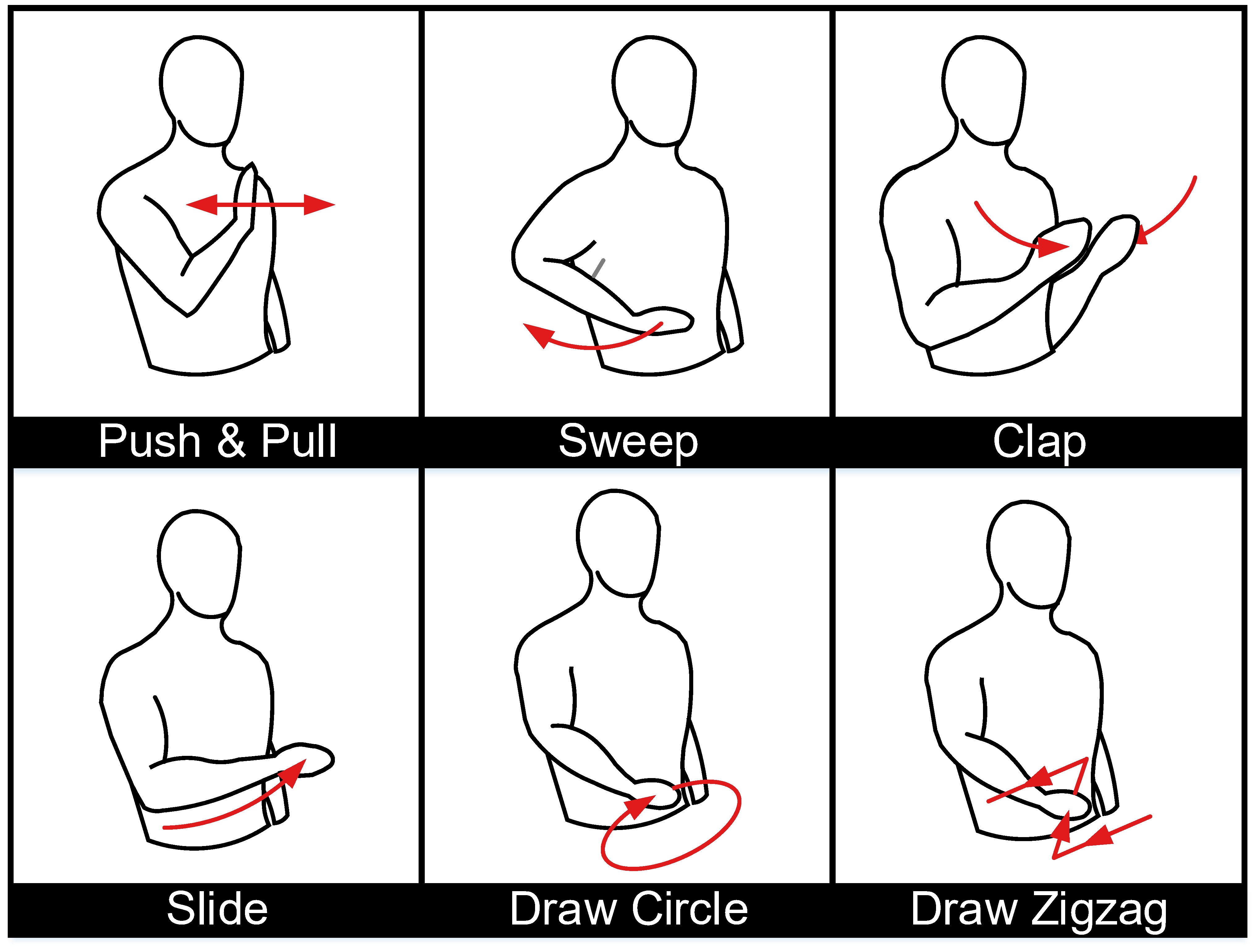 Fig. 9. Sketches of gestures evaluated in the experiment.
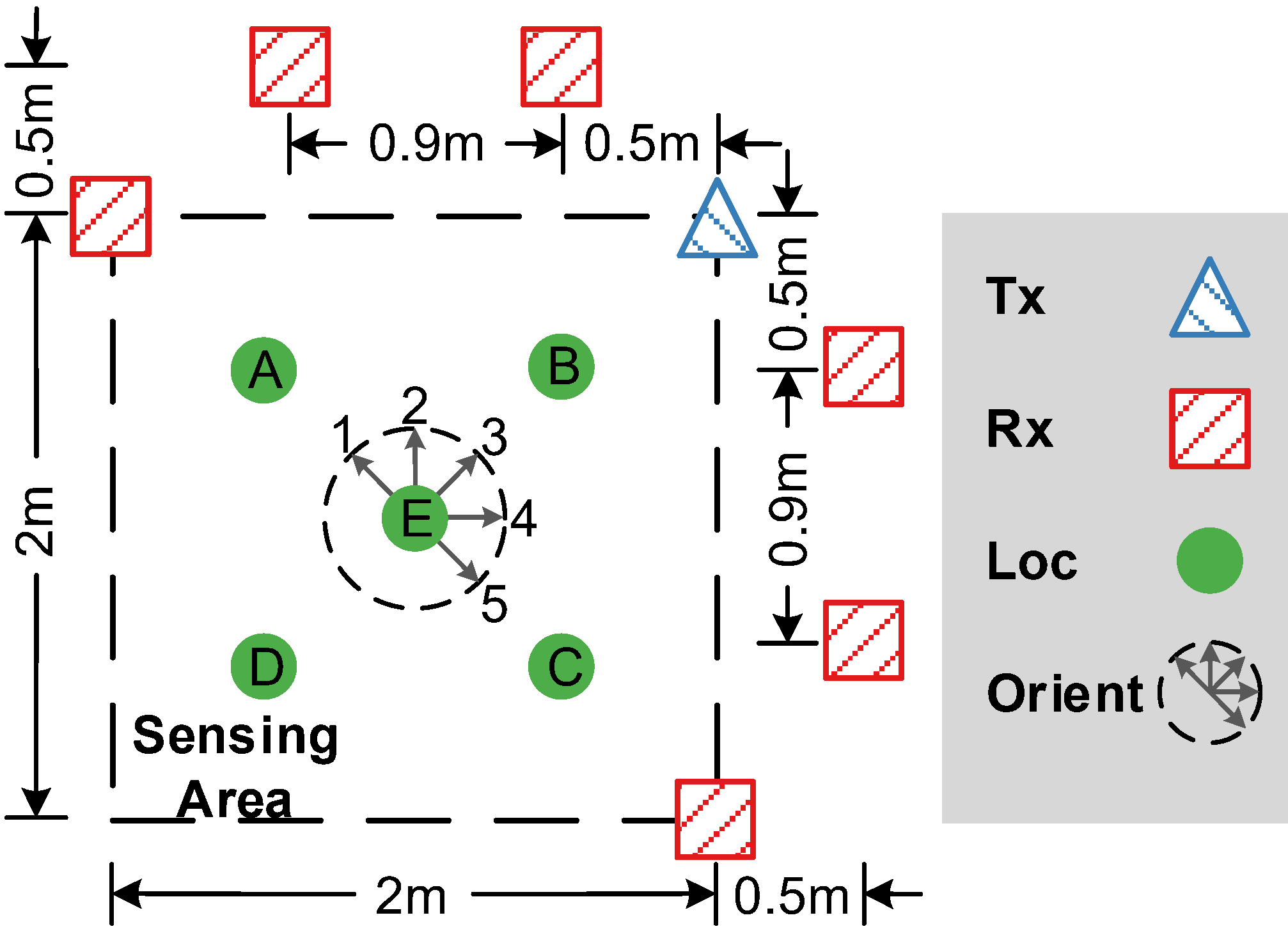 Fig. 10. The setup of Wi-Fi devices for gesture recognition task.
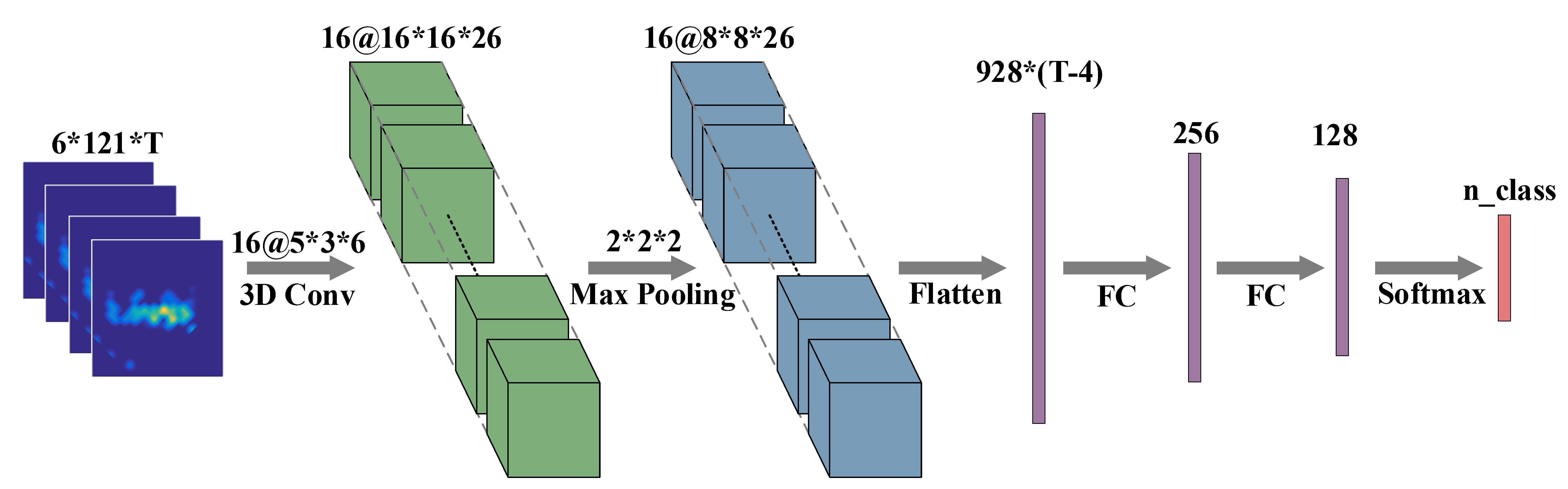 Fig. 11. Convolutional Neural Network architecture.
We now introduce the implementation code in detail.
First, some necessary packages are imported. We use Keras 5 API with TensorFlow as the backend to demonstrate how to implement the neural network.
import os,sys
import numpy as np
import scipy.io as scio
import tensorflow as tf
import keras
from keras.layers import Input, GRU, Dense, Flatten, Dropout, Conv2D, Conv3D, MaxPooling2D, MaxPooling3D, TimeDistributed, Bidirectional, Multiply, Permute, RepeatVector, Concatenate, Dot, Lambda
from keras.models import Model, load_model
import keras.backend as K
from sklearn.metrics import confusion_matrix
from keras.backend.tensorflow_backend import set_session
from sklearn.model_selection import train_test_split
Then we define some parameters, including the hyperparameters and the data path. The fraction of testing data is defined as 0.1. To simplify the problem, we only use six gesture types in the widar3.0 dataset.
# Parameters
fraction_for_test = 0.1
data_dir = 'widar30dataset/DFS/20181130/'
ALL_MOTION = [1,2,3,4,5,6]
N_MOTION = len(ALL_MOTION)
T_MAX = 0
n_epochs = 200
f_dropout_ratio = 0.5
n_gru_hidden_units = 64
n_batch_size = 32
f_learning_rate = 0.001
The program begins with loading data with the predefined function load_data. The loaded data are split into train and test by calling the API function train_test_split. The labels of the training data are encoded into the one-hot format with the predefined function onehot_encoding.
# Load data
data, label = load_data(data_dir)
print('\nLoaded dataset of ' + str(label.shape[0]) + ' samples, each sized ' + str(data[0,:,:,:,:].shape) + '\n')

# Split train and test
[data_train, data_test, label_train, label_test] = train_test_split(data, label, test_size=fraction_for_test)
print('\nTrain on ' + str(label_train.shape[0]) + ' samples\n' +\
    'Test on ' + str(label_test.shape[0]) + ' samples\n')

# One-hot encoding for train data
label_train = onehot_encoding(label_train, N_MOTION)
After loading and formatting the training and testing data, we defined the model with the predefined function \lstinline{build_model}. After that, we train the model by calling the API function \lstinline{fit}. The input data and label are specified in the parameters. The fraction of validation data is specified as 0.1.
model = build_model(input_shape=(T_MAX, 6, 121, 1), n_class=N_MOTION)
model.summary()
model.fit({'name_model_input': data_train},{'name_model_output': label_train},
        batch_size=n_batch_size,
        epochs=n_epochs,
        verbose=1,
        validation_split=0.1, shuffle=True)
After the training process, we evaluate the model with the test dataset. The predictions are converted from one-hot format to integers and are used to calculate the confusion matrix and accuracy.
# Testing...
print('Testing...')
label_test_pred = model.predict(data_test)
label_test_pred = np.argmax(label_test_pred, axis = -1) + 1

# Confusion Matrix
cm = confusion_matrix(label_test, label_test_pred)
print(cm)
cm = cm.astype('float')/cm.sum(axis=1)[:, np.newaxis]
cm = np.around(cm, decimals=2)
print(cm)

# Accuracy
test_accuracy = np.sum(label_test == label_test_pred) / (label_test.shape[0])
print(test_accuracy)
The predefined onehot_encoding function convert the label to one-hot format.
def onehot_encoding(label, num_class):
    # label(ndarray)=>_label(ndarray): [N,]=>[N,num_class]
    label = np.array(label).astype('int32')
    label = np.squeeze(label)
    _label = np.eye(num_class)[label-1]
    return _label
The predefined load_data function is used to load all data samples and labels from a directory.
Each file in the directory corresponds to a single data sample.
Each data sample is normalized with the predefined normalize_data function.
It is worth noting that the data samples have different time durations.
We use a predefined zero_padding function to make their durations the same as the longest one.
def load_data(path_to_data):
    global T_MAX
    data = []
    label = []
    for data_root, data_dirs, data_files in os.walk(path_to_data):
        for data_file_name in data_files:

            file_path = os.path.join(data_root,data_file_name)
            try:
                data_1 = scio.loadmat(file_path)['doppler_spectrum']    # [6,121,T]
                label_1 = int(data_file_name.split('-')[1])
                location = int(data_file_name.split('-')[2])
                orientation = int(data_file_name.split('-')[3])
                repetition = int(data_file_name.split('-')[4])

                # Downsample
                data_1 = data_1[:,:,0::10]

                # Select Motion
                if (label_1 not in ALL_MOTION):
                    continue

                # Normalization
                data_normed_1 = normalize_data(data_1)

                # Update T_MAX
                if T_MAX < np.array(data_1).shape[2]:
                    T_MAX = np.array(data_1).shape[2]
            except Exception:
                continue

            # Save List
            data.append(data_normed_1.tolist())
            label.append(label_1)

    # Zero-padding
    data = zero_padding(data, T_MAX)

    # Swap axes
    data = np.swapaxes(np.swapaxes(data, 1, 3), 2, 3)   # [N,6,121,T_MAX]=>[N,T_MAX,6,121]
    data = np.expand_dims(data, axis=-1)                # [N,T_MAX,6,121]=>[N,T_MAX,6,121,1]

    # Convert label to ndarray
    label = np.array(label)

    # data(ndarray): [N,T_MAX,6,121,1], label(ndarray): [N,]
    return data, label
The normalize_data function is used to normalize the loaded data samples.
Each data sample has a dimension of , in which the number "6" represents the number of Wi-Fi receivers, the number "121" represents the frequency bins, and the "T" represents the time durations.
To normalize a sample, we scale the data to be in the range of for each time snapshot.
def normalize_data(data_1):
    # data(ndarray)=>data_norm(ndarray): [6,121,T]=>[6,121,T]
    data_1_max = np.amax(data_1,(0,1),keepdims=True)    # [6,121,T]=>[1,1,T]
    data_1_min = np.amin(data_1,(0,1),keepdims=True)    # [6,121,T]=>[1,1,T]
    data_1_max_rep = np.tile(data_1_max,(data_1.shape[0],data_1.shape[1],1))    # [1,1,T]=>[6,121,T]
    data_1_min_rep = np.tile(data_1_min,(data_1.shape[0],data_1.shape[1],1))    # [1,1,T]=>[6,121,T]
    data_1_norm = (data_1 - data_1_min_rep) / (data_1_max_rep - data_1_min_rep + sys.float_info.min)
    return  data_1_norm
The zero_padding function is used to align all the data samples to have the same duration. The padded length is specified by the parameter T_MAX.
def zero_padding(data, T_MAX):
    # data(list)=>data_pad(ndarray): [6,121,T1/T2/...]=>[6,121,T_MAX]
    data_pad = []
    for i in range(len(data)):
        t = np.array(data[i]).shape[2]
        data_pad.append(np.pad(data[i], ((0,0),(0,0),(T_MAX - t,0)), 'constant', constant_values = 0).tolist())
    return np.array(data_pad)
In this function, we define the network structure.
The input layer is specified with the API function Input, which has the parameters to define the input shape, data type, and the layer name.
Following the input layer, we use a three-dimensional convolutional layer, a max-pooling layer, and two fully connected layers.
The output layer is specified with the API function Output, which has the parameters to define the activation function, the dimension, and the name.
At last, we finalize the model with the API function Model and compile.
The optimizer is specified to \lstinline{RMSprop}, and the loss is specified to categorical_crossentropy.
def build_model(input_shape, n_class):
    model_input = Input(shape=input_shape, dtype='float32', name='name_model_input')    # (@,T_MAX,6,121,1)

    # CNN
    x = Conv3D(16,kernel_size=(5,3,6),activation='relu',data_format='channels_last',\
        input_shape=input_shape)(model_input)   # (@,T_MAX-4,6,121,1)=>(@,T_MAX-4,4,116,16)
    x = MaxPooling3D(pool_size=(2,2,2))(x)      # (@,T_MAX-4,4,116,16)=>(@,T_MAX-4,2,58,16)

    x = Flatten()(x)                            # (@,T_MAX-4,2,58,16)=>(@,(T_MAX-4)*2*58*16)
    x = Dense(256,activation='relu')(x)         # (@,(T_MAX-4)*2*58*16)=>(@,256)
    x = Dropout(f_dropout_ratio)(x)
    x = Dense(128,activation='relu')(x)         # (@,256)=>(@,128)
    x = Dropout(f_dropout_ratio)(x)
    model_output = Dense(n_class, activation='softmax', name='name_model_output')(x)  # (@,128)=>(@,n_class)

    # Model compiling
    model = Model(inputs=model_input, outputs=model_output)
    model.compile(optimizer=keras.optimizers.RMSprop(lr=f_learning_rate),
                    loss='categorical_crossentropy',
                    metrics=['accuracy']
                )
    return model
Recurrent Neural Network
Recurrent Neural Network (RNN) is designed for modeling temporal dynamics of sequences and is commonly used for time series data analysis like speech recognition and natural language processing. Wireless signals are highly correlated over time and can be processed with RNN. Some works 1 3 have demonstrated the potential of RNN for wireless sensing tasks. In this section, we will present a working example of combining CNN and RNN to perform gesture recognition with Wi-Fi. The experimental settings are the same as in \sect{sec:cnn}. We also extract DFS from the raw CSI as the input feature of the network. The network architecture is shown in Figure. 12.
We now introduce the implementation code in detail.
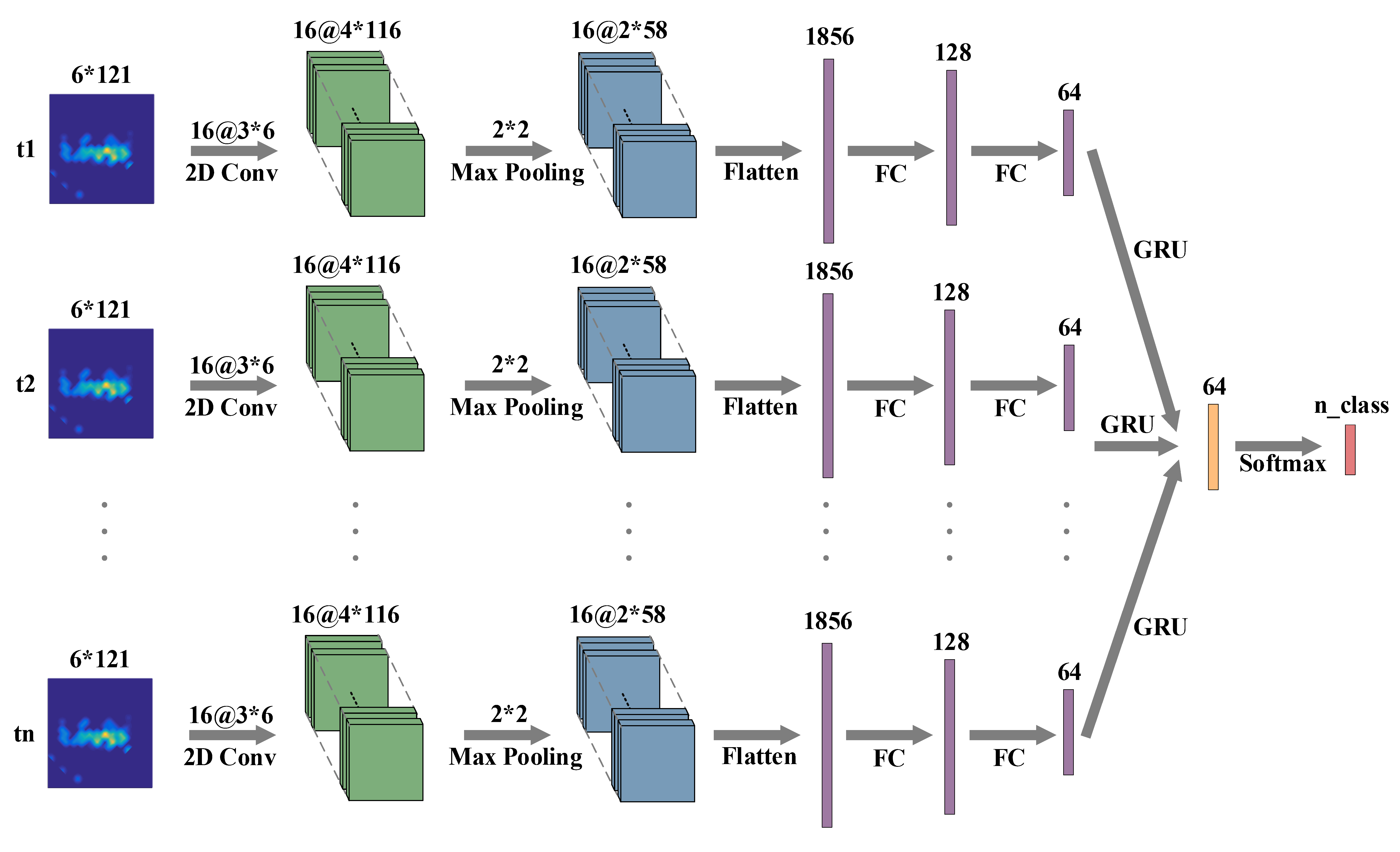 Fig. 12. Recurrent Neural Network architecture.
Most of the code is the same as in \sect{sec:cnn} except for the model definition. To define the model, we use two-dimensional convolutional layer and max-pooling layer on the dimensional except for the time dimension of the data. We adopt the GRU layer as the recurrent layer.
def build_model(input_shape, n_class):
    model_input = Input(shape=input_shape, dtype='float32', name='name_model_input')    # (@,T_MAX,6,121,1)

    # CNN+RNN
    x = TimeDistributed(Conv2D(16,kernel_size=(3,6),activation='relu',data_format='channels_last',\
        input_shape=input_shape))(model_input)              # (@,T_MAX,6,121,1)=>(@,T_MAX,4,116,16)
    x = TimeDistributed(MaxPooling2D(pool_size=(2,2)))(x)   # (@,T_MAX,4,116,16)=>(@,T_MAX,2,58,16)

    x = TimeDistributed(Flatten())(x)                       # (@,T_MAX,2,58,16)=>(@,T_MAX,2*58*16)
    x = TimeDistributed(Dense(128,activation='relu'))(x)    # (@,T_MAX,2*58*16)=>(@,T_MAX,128)
    x = TimeDistributed(Dropout(f_dropout_ratio))(x)
    x = TimeDistributed(Dense(64,activation='relu'))(x)     # (@,T_MAX,128)=>(@,T_MAX,64)

    x = GRU(n_gru_hidden_units,return_sequences=False)(x)   # (@,T_MAX,64)=>(@,64)
    x = Dropout(f_dropout_ratio)(x)
    model_output = Dense(n_class, activation='softmax', name='name_model_output')(x)  # (@,64)=>(@,n_class)

    # Model compiling
    model = Model(inputs=model_input, outputs=model_output)
    model.compile(optimizer=keras.optimizers.RMSprop(lr=f_learning_rate),
                    loss='categorical_crossentropy',
                    metrics=['accuracy']
                )
    return model
Adversarial Learning
Except for the basic neural network components, some high-level network architectures also play essential roles in wireless sensing. Similar to computer vision tasks, wireless sensing also suffer from domain misalignment problem. Wireless signals can be reflected by the surrounding objects during propagation and will be flooded with target-irrelevant signal components. The sensing system trained in one deployment environment can hardly be applied directly in other settings without adaptation. Some works 6 try to adopt adversarial learning techniques to tackle this problem and achieve promising performance. This section will give an example of how to apply this technique in wireless sensing tasks. Specifically, we build a gesture recognition system with Wi-Fi, similar to that in \sect{sec:cnn}. We try to achieve consistent performance across different human locations and orientations. The network architecture is shown in Figure. 13.
We now introduce the implementation code in detail.
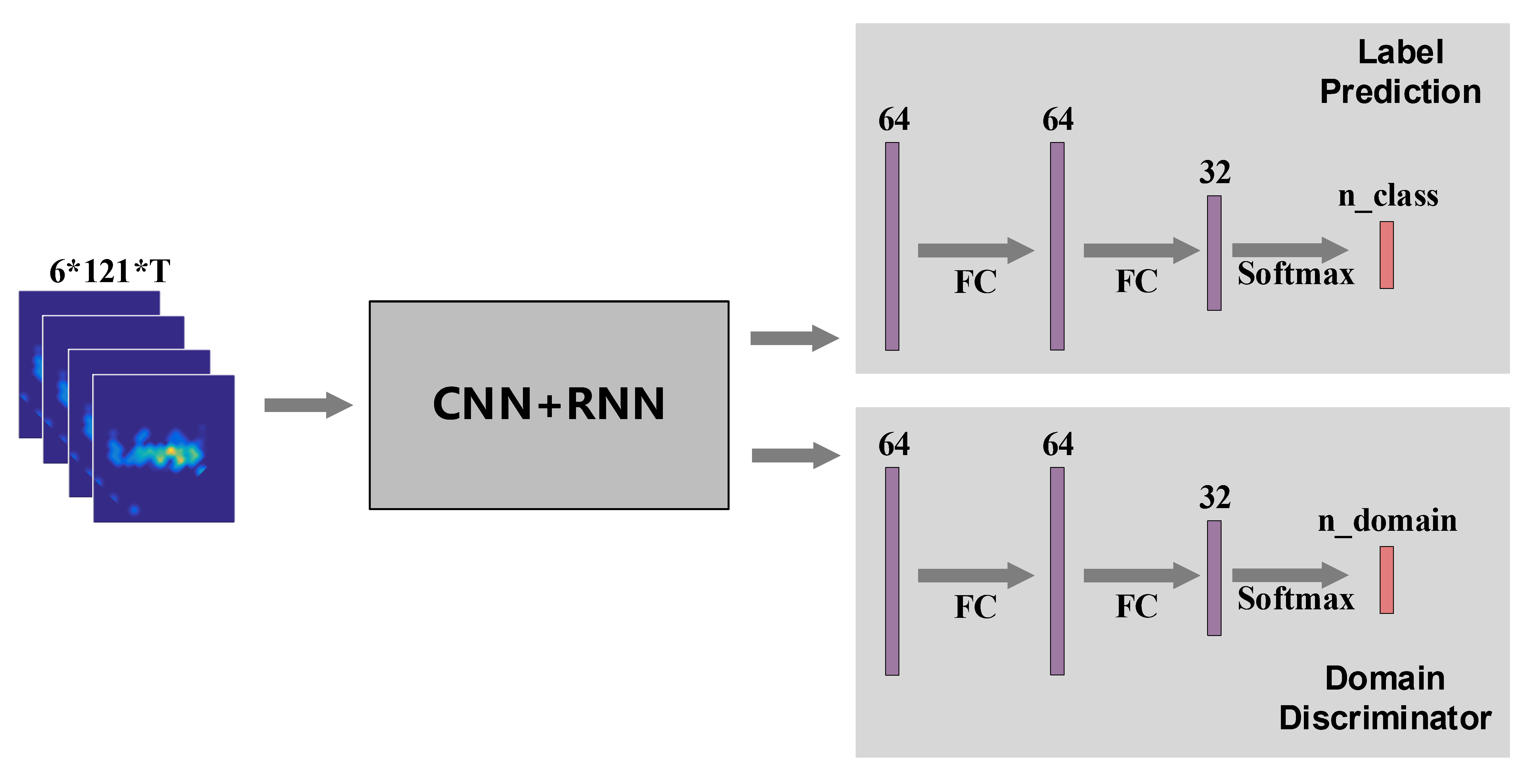 Fig. 13. Adversarial learning network architecture.
In the Widar3.0 dataset 4, we collect gesture data when the users stand at different locations. As discussed in \sect{sec:DFS}, human locations have significant impact on the DFS measurements. To mitigate this impact, we treat human locations as different domains and build an adversarial learning network to recognize gestures irrespective of domains. In the program, we first load data, labels, and domains from the dataset and split them into train and test. Both label and domain are encoded into the one-hot format.
# Load data
data, label, domain = load_data(data_dir)
print('\nLoaded dataset of ' + str(label.shape[0]) + ' samples, each sized ' + str(data[0,:,:,:,:].shape) + '\n')

# Split train and test
[data_train, data_test, label_train, label_test, domain_train, domain_test] = train_test_split(data, label, domain, test_size=fraction_for_test)
print('\nTrain on ' + str(label_train.shape[0]) + ' samples\n' +\
    'Test on ' + str(label_test.shape[0]) + ' samples\n')

# One-hot encoding for train data
label_train = onehot_encoding(label_train, N_MOTION)
domain_train = onehot_encoding(domain_train, N_LOCATION)
After loading and formating data, we built the network and trained it from scratch.
The training data, label, and domain are passed to the API function fit for training.
# Train Model
model = build_model(input_shape=(T_MAX, 6, 121, 1), n_class=N_MOTION, n_domain=N_LOCATION)
model.summary()
model.fit({'name_model_input': data_train},{'name_model_output_label': label_train, 'name_model_output_domain': domain_train},
        batch_size=n_batch_size,
        epochs=n_epochs,
        verbose=1,
        validation_split=0.1, shuffle=True)
After the training process finishes, we evaluate the network with the test samples. Note that the adversarial network has both label and domain prediction outputs. We only use the label output for accuracy evaluation.
# Testing...
print('Testing...')
[label_test_pred,_] = model.predict(data_test)
label_test_pred = np.argmax(label_test_pred, axis = -1) + 1

# Confusion Matrix
cm = confusion_matrix(label_test, label_test_pred)
print(cm)
cm = cm.astype('float')/cm.sum(axis=1)[:, np.newaxis]
cm = np.around(cm, decimals=2)
print(cm)

# Accuracy
test_accuracy = np.sum(label_test == label_test_pred) / (label_test.shape[0])
print(test_accuracy)
Different from that in \sect{sec:cnn}, we load data, label, and domain in the load_data function.
The domain is defined as the location of the human, which is embedded in the file name.
def load_data(path_to_data):
    global T_MAX
    data = []
    label = []
    domain = []
    for data_root, data_dirs, data_files in os.walk(path_to_data):
        for data_file_name in data_files:

            file_path = os.path.join(data_root,data_file_name)
            try:
                data_1 = scio.loadmat(file_path)['doppler_spectrum']    # [6,121,T]
                label_1 = int(data_file_name.split('-')[1])
                location_1 = int(data_file_name.split('-')[2])
                orientation_1 = int(data_file_name.split('-')[3])
                repetition_1 = int(data_file_name.split('-')[4])

                # Downsample
                data_1 = data_1[:,:,0::10]

                # Select Motion
                if (label_1 not in ALL_MOTION):
                    continue

                # Normalization
                data_normed_1 = normalize_data(data_1)

                # Update T_MAX
                if T_MAX < np.array(data_1).shape[2]:
                    T_MAX = np.array(data_1).shape[2]
            except Exception:
                continue

            # Save List
            data.append(data_normed_1.tolist())
            label.append(label_1)
            domain.append(location_1)

    # Zero-padding
    data = zero_padding(data, T_MAX)

    # Swap axes
    data = np.swapaxes(np.swapaxes(data, 1, 3), 2, 3)   # [N,6,121,T_MAX]=>[N,T_MAX,6,121]
    data = np.expand_dims(data, axis=-1)                # [N,T_MAX,6,121]=>[N,T_MAX,6,121,1]

    # Convert label and domain to ndarray
    label = np.array(label)
    domain = np.array(domain)

    # data(ndarray): [N,T_MAX,6,121,1], label(ndarray): [N,], domain(ndarray): [N,]
    return data, label, domain
To define the network, we use a CNN layer and an RNN layer as the feature extractor, which is similar to that in \sect{sec:rnn}.
In the gesture recognizer and domain discriminator, we use two fully-connected layers and an output layer activated by softmax function, respectively.
We use categorical cross-entropy loss for both label prediction and domain prediction outputs.
The domain prediction loss is weighted with loss_weight_domain and subtracted from the label prediction loss.
def build_model(input_shape, n_class, n_domain):
    model_input = Input(shape=input_shape, dtype='float32', name='name_model_input')    # (@,T_MAX,6,121,1)

    # CNN+RNN+Adversarial
    x = TimeDistributed(Conv2D(16,kernel_size=(3,6),activation='relu',data_format='channels_last',\
        input_shape=input_shape))(model_input)              # (@,T_MAX,6,121,1)=>(@,T_MAX,4,116,16)
    x = TimeDistributed(MaxPooling2D(pool_size=(2,2)))(x)   # (@,T_MAX,4,116,16)=>(@,T_MAX,2,58,16)

    x = TimeDistributed(Flatten())(x)                       # (@,T_MAX,2,58,16)=>(@,T_MAX,2*58*16)
    x = TimeDistributed(Dense(128,activation='relu'))(x)    # (@,T_MAX,2*58*16)=>(@,T_MAX,128)
    x = TimeDistributed(Dropout(f_dropout_ratio))(x)
    x = TimeDistributed(Dense(64,activation='relu'))(x)     # (@,T_MAX,128)=>(@,T_MAX,64)

    x = GRU(n_gru_hidden_units,return_sequences=False)(x)   # (@,T_MAX,64)=>(@,64)
    x_feat = Dropout(f_dropout_ratio)(x)

    # Label prediction part
    x_1 = Dense(64, activation='relu')(x_feat)      # (@,64)=>(@,64)
    x_1 = Dense(32, activation='relu')(x_1)         # (@,64)=>(@,32)
    model_output_label = Dense(n_class, activation='softmax', name='name_model_output_label')(x_1)      # (@,32)=>(@,n_class)

    # Domain prediction part
    x_2 = Dense(64, activation='relu')(x_feat)      # (@,64)=>(@,64)
    x_2 = Dense(32, activation='relu')(x_2)         # (@,64)=>(@,32)
    model_output_domain = Dense(n_domain, activation='softmax', name='name_model_output_domain')(x_2)   # (@,32)=>(@,n_domain)


    model = Model(inputs=model_input, outputs=[model_output_label, model_output_domain])
    model.compile(optimizer=keras.optimizers.RMSprop(lr=f_learning_rate),
            loss = {'name_model_output_label':custom_loss_label(), 'name_model_output_domain':custom_loss_domain()},
            loss_weights={'name_model_output_label':1, 'name_model_output_domain':-1*loss_weight_domain},
            metrics={'name_model_output_label':'accuracy', 'name_model_output_domain':'accuracy'}
            )

    return model
The pre-defined custom_loss_label and custom_loss_domain are categorical crossentropy losses for both label prediction and domain prediction.
def custom_loss_label():
    def lossfn(y_true, y_pred):
        myloss_batch = -1 * K.sum(y_true*K.log(y_pred+K.epsilon()), axis=-1, keepdims=False)
        myloss = K.mean(myloss_batch, axis=-1, keepdims=False)
        return myloss
    return lossfn
def custom_loss_domain():
    def lossfn(y_true, y_pred):
        myloss_batch = -1 * K.sum(y_true*K.log(y_pred+K.epsilon()), axis=-1, keepdims=False)
        myloss = K.mean(myloss_batch, axis=-1, keepdims=False)
        return myloss
    return lossfn
Complex-valued Neural Network
In this section, we will present a more complicated wireless sensing task with deep learning. Many wireless sensing approaches employ Fast Fourier Transform (FFT) on a time series of RF data to obtain time-frequency spectrograms of human activities. FFT suffers from errors due to an effect known as leakage, when the block of data is not periodic (the most common case in practice), which results in a smeared spectrum of the original signal and further leads to misleading data representation for learning-based sensing. Classical approaches reduce leakage by windowing, which cannot eliminate leakage entirely. Considering the significant fitting capability of deep neural networks, we can design a signal processing network to learn an optimal function to minimize or nearly eliminate the leakage and enhance the spectrums, which we call the Signal Enhancement Network (SEN).
The signal processing network takes as input a spectrogram transformed from wireless signals via STFT, removes the spectral leakage in the spectrogram, and recovers the underlying actual frequency components. Figure. 17 shows the training process of the network. As shown in the upper part of Figure. 17, we randomly generate ideal spectrums with 1 to 5 frequency components, whose amplitudes, phases, and frequencies are uniformly drawn from their ranges of interest. Then, the ideal spectrum is converted to the leaked spectrum following the process in the following equation to simulate the windowing effect and random complex noises:
where and are the ideal and estimated frequency spectrum, respectively, represents the additive Gaussian noise vector, and is the convolution matrix of the windowing function in the frequency domain. The column of is:
where represents the windowing function of FFT in time domain.
The amplitude of the noise follows a Gaussian distribution and its phase follows a uniform distribution in . The network takes the leaked spectrum as input and outputs the enhanced spectrum close to the ideal one. Thus, we minimize the loss during training. During inference, the spectrums measured from real-world scenarios are normalized to and fed into the network to obtain the enhanced spectrum.
We now present the implementation code in detail.
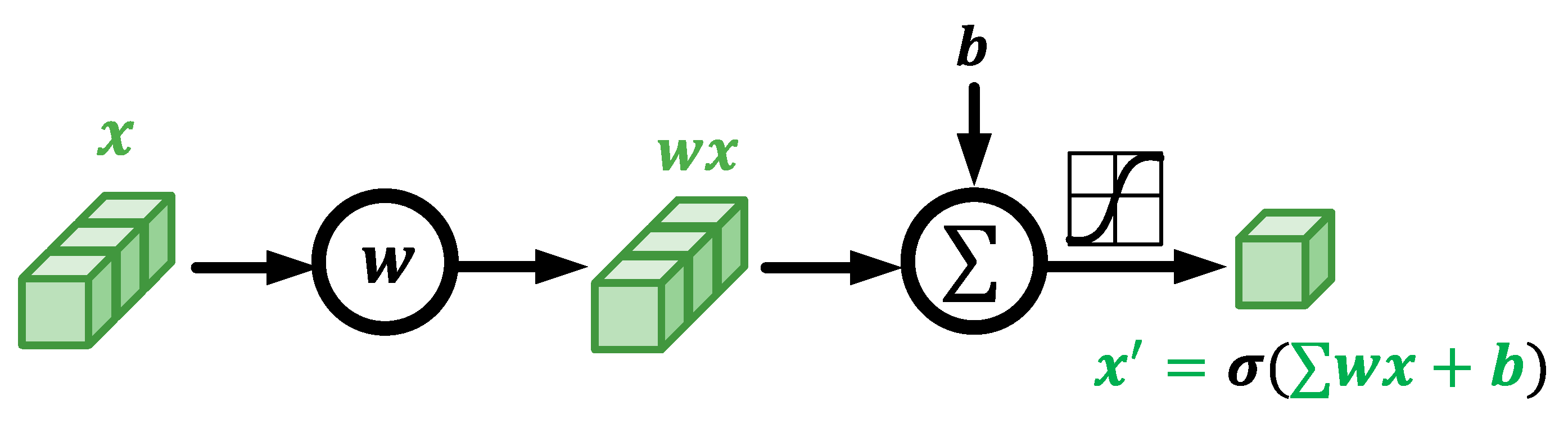 Fig. 14. Real-valued neurons.
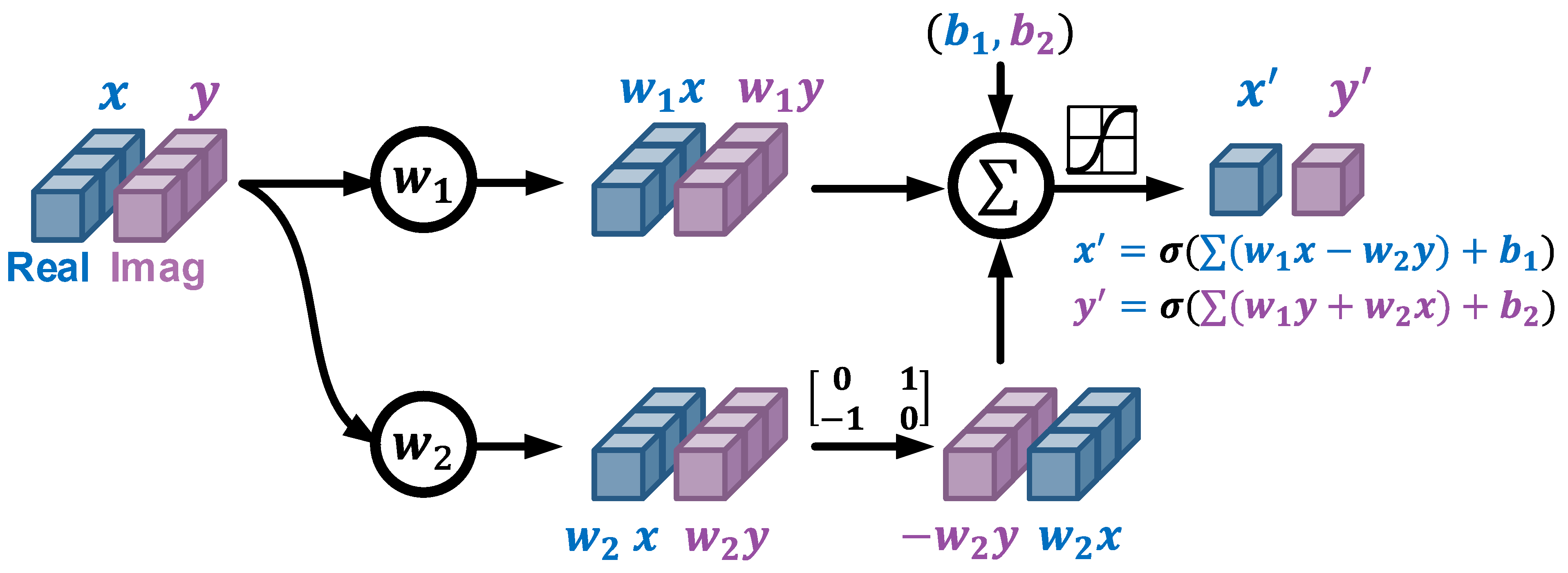 Fig. 15. Complex-valued neurons.
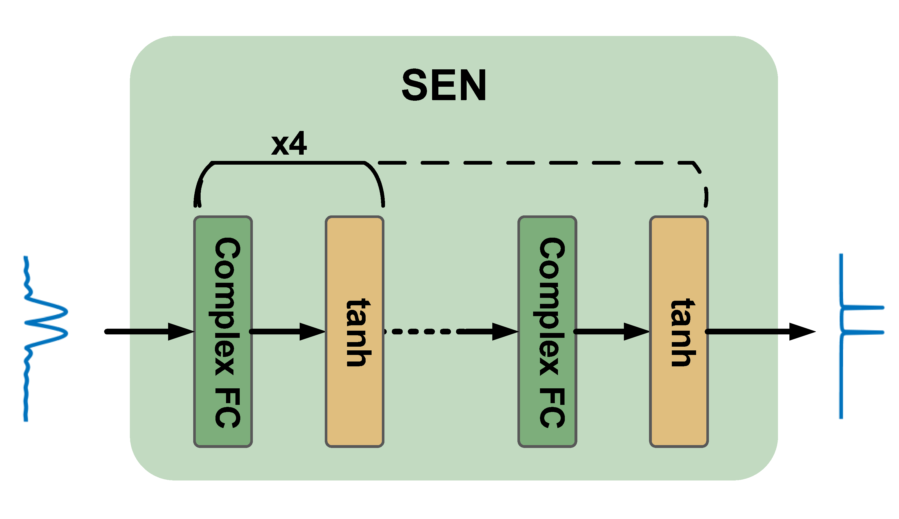 Fig. 16. Complex-valued neural network architecture.
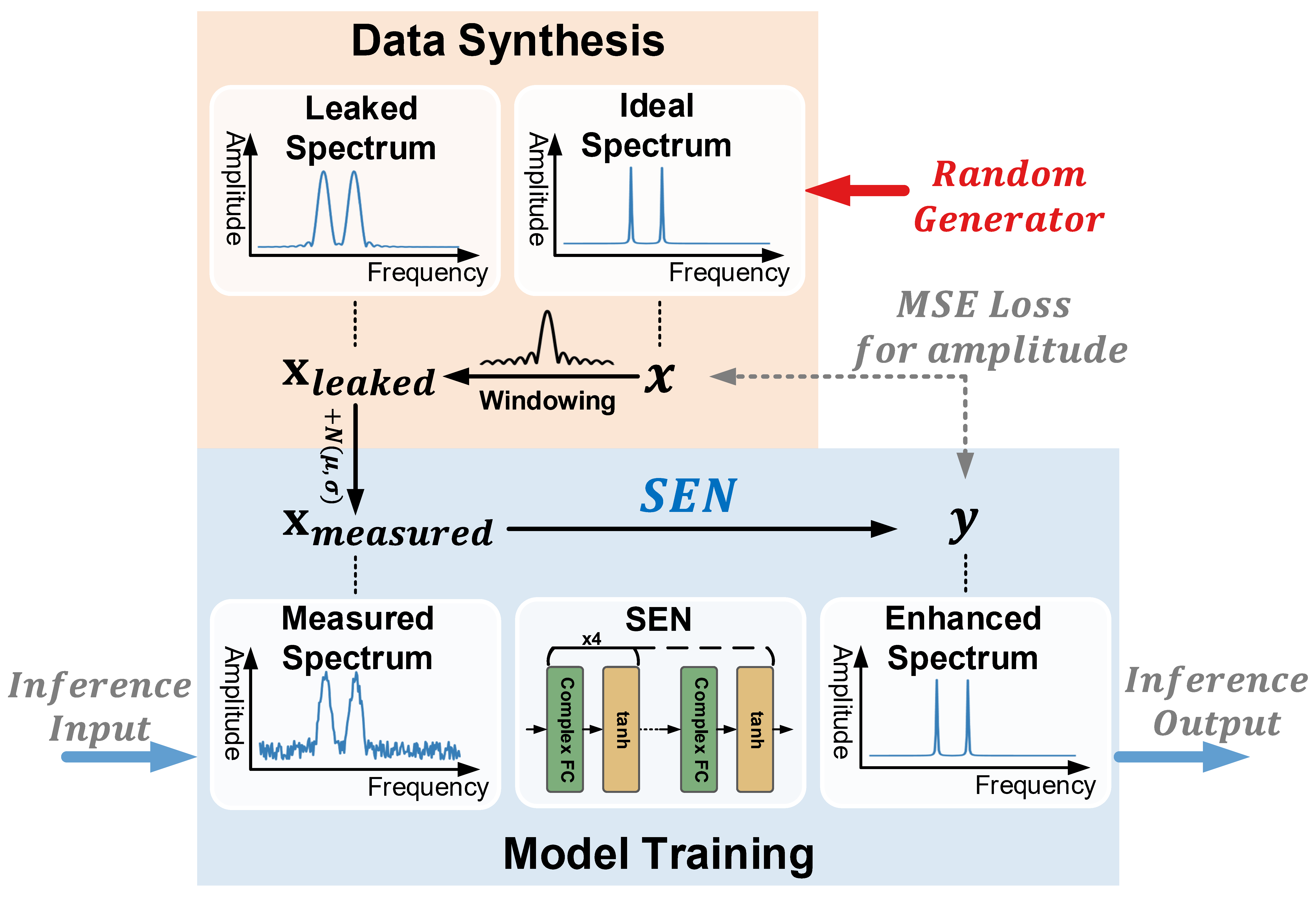 Fig. 17. The training process of the signal processing network.
Different from previous sections, we use the PyTorch platform to implement the network. PyTorch provides the interface to implement custom layers, which makes the implementation of the CVNN much more convenient. We first import some necessary packages as follows.
import os,sys,math,scipy,imp
import numpy as np
import scipy.io as scio
import torch, torchvision
import torch.nn as nn
from scipy import signal
from math import sqrt,log,pi
from torch.fft import fft,ifft
from torch.nn.functional import relu, softmax, cross_entropy
from torch import sigmoid,tanh
from torch.nn import MSELoss as MSE
Some parameters are defined in this part.
# Definition
wind_len = 125
wind_type = 'gaussian'
n_max_freq_component = 3
AWGN_amp = 0.01
str_modelname_prefix = './SEN_Results/SEN_' + wind_type + '_W' + str(wind_len)
str_model_name_pretrained = str_modelname_prefix + '_E1000.pt'
feature_len = 121
padded_len = 1000
crop_len = feature_len
blur_matrix_left = []

# Hyperparameters
n_begin_epoch = 1
n_epoch = 10000
n_itr_per_epoch = 500
n_batch_size = 64
n_test_size = 200
f_learning_rate = 0.001
The program begins with the following code.
We first generate the convolution matrix of the windowing function (Eqn.36) with the pre-defined function generate_blur_matrix_complex, which will be introduced shortly.
Then we define the SEN model and move it to the GPU processor with the API function cuda.
After the model definition, we train the model with synthetic spectrograms, during which process we save the trained model every 500 epochs.
The trained and saved model can be directly loaded and used to enhance spectrograms.
if __name__ == "__main__":
    # Generate blur matrix
    blur_matrix_right = generate_blur_matrix_complex(wind_type=wind_type, wind_len=wind_len, padded_len=padded_len, crop_len=crop_len)

    # Define model
    print('Model building...')
    model = SEN(feature_len=feature_len)
    model.cuda()

    # Train model
    print('Model training...')
    train(model=model, blur_matrix_right=blur_matrix_right, feature_len=feature_len, n_epoch=n_epoch, n_itr_per_epoch=n_itr_per_epoch, n_batch_size=n_batch_size, optimizer=torch.optim.RMSprop(model.parameters(), lr=f_learning_rate))
This generate_blur_matrix_complex function is used to generate the convolution matrix of the windowing function.
The core idea behind this function is to enumerate all the frequencies, apply the window function on the sinusoid signal, and generate the corresponding spectrums with FFT.
After obtaining the convolution matrix, we can bridge the gap between the ideal and the leaked spectrograms with Eqn.35.
In other words, we can directly get the leaked spectrograms by multiplying the idea spectrograms with the convolution matrix.
def generate_blur_matrix_complex(wind_type, wind_len=251, padded_len=1000, crop_len=121):
    # Generate matrix used to introduce spec leakage in complex domain
    # ret: (ndarray.complex128) [crop_len, crop_len](row first)
    # Row first: each row represents the spectrum of one single carrier

    # Steps: carrier/windowing/pad/fft/crop/unwrap/norm

    # Parameters offloading
    fs = 1000
    n_f_bins = crop_len
    f_high = int(n_f_bins/2)
    f_low = -1 * f_high
    init_phase = 0

    # Carrier
    t_ = np.arange(0,wind_len).reshape(1,wind_len)/fs       # [1,wind_len] (0~wind_len/fs seconds)
    freq = np.arange(f_low,f_high+1,1).reshape(n_f_bins,1)  # [n_f_bins,1] (f_low~f_high Hz)
    phase = 2 * pi * freq * t_ + init_phase                 # [n_f_bins,wind_len]
    signal = np.exp(1j*phase)                               # [n_f_bins,wind_len]~[121,251]

    # Windowing
    if wind_type == 'gaussian':
        window = scipy.signal.windows.gaussian(wind_len, (wind_len-1)/sqrt(8*log(200)), sym=True)   # [wind_len,]
    else:
        window = scipy.signal.get_window(wind_type, wind_len)
    sig_wind = signal * window       # [n_f_bins,wind_len]*[wind_len,]=[n_f_bins,wind_len]~[121,251]

    # Pad/FFT
    sig_wind_pad = np.concatenate((sig_wind, np.zeros((n_f_bins,padded_len-wind_len))),axis=1)  # [n_f_bins,wind_len]=>[n_f_bins,padded_len]
    sig_wind_pad_fft = np.fft.fft(sig_wind_pad, axis=-1)    # [n_f_bins,padded_len]~[121,1000]

    # Crop
    n_freq_pos = f_high + 1
    n_freq_neg = abs(f_low)
    sig_wind_pad_fft_crop = np.concatenate((sig_wind_pad_fft[:,:n_freq_pos],\
        sig_wind_pad_fft[:,-1*n_freq_neg:]), axis=1)      # [n_f_bins,crop_len]~[121,121]

    # Unwrap
    n_shift = n_freq_neg
    sig_wind_pad_fft_crop_unwrap = np.roll(sig_wind_pad_fft_crop, shift=n_shift, axis=1) # [n_f_bins,crop_len]~[121,121]

    # Norm (amp_max=1)
    _sig_amp = np.abs(sig_wind_pad_fft_crop_unwrap)
    _sig_ang = np.angle(sig_wind_pad_fft_crop_unwrap)
    _max = np.tile(_sig_amp.max(axis=1,keepdims=True), (1,crop_len))
    _min = np.tile(_sig_amp.min(axis=1,keepdims=True), (1,crop_len))
    _sig_amp_norm = _sig_amp / _max
    sig_wind_pad_fft_crop_unwrap_norm = _sig_amp_norm * np.exp(1j*_sig_ang)

    # Return
    ret = sig_wind_pad_fft_crop_unwrap_norm

    return ret
This function is to generate one batch of spectrograms in both the leaked form and the idea form. The process is the same as that illustrated in Eqn.35.
def syn_one_batch_complex(blur_matrix_right, feature_len, n_batch):
    # Syn. HiFi, blurred and AWGN signal in complex domain
    # ret: (ndarray.complex128) [@,feature_len]
    # blur_matrix_right: Row first (each row represents the spectrum of one single carrier)

    # Syn. x [@,feature_len]
    x = np.zeros((n_batch, feature_len))*np.exp(1j*0)
    for i in range(n_batch):
        num_carrier = int(np.random.randint(0,n_max_freq_component,1))
        idx_carrier = np.random.permutation(feature_len)[:num_carrier]
        x[i,idx_carrier] = np.random.rand(1,num_carrier) * np.exp(1j*( 2*pi*np.random.rand(1,num_carrier) - pi ))

    # Syn. x_blur [@,feature_len]
    x_blur = x @ blur_matrix_right

    # Syn. x_tilde [@,feature_len]
    x_tilde = x_blur + 2*AWGN_amp*(np.random.random(x_blur.shape)-0.5) *\
        np.exp(1j*( 2*pi*np.random.random(x_blur.shape) - pi ))

    return x, x_blur, x_tilde
This part demonstrates the code on how to implement the SEN network.
According to the API of PyTorch, both the __init__ and the forward interfaces should be implemented with customized algorithms.
In the __init__ function, we defined five complex-valued fully-connected layers.
In the forward function, we defined the network structure by concatenating the five FC layers and specifying the input and output layers.
class SEN(nn.Module):
    def __init__(self, feature_len):
        super(SEN, self).__init__()
        self.feature_len = feature_len

        self.fc_1 = m_Linear(feature_len, feature_len)
        self.fc_2 = m_Linear(feature_len, feature_len)
        self.fc_3 = m_Linear(feature_len, feature_len)
        self.fc_4 = m_Linear(feature_len, feature_len)
        self.fc_out = m_Linear(feature_len, feature_len)

    def forward(self, x):
        h = x   # (@,*,2,H)

        h = tanh(self.fc_1(h))          # (@,*,2,H)=>(@,*,2,H)
        h = tanh(self.fc_2(h))          # (@,*,2,H)=>(@,*,2,H)
        h = tanh(self.fc_3(h))          # (@,*,2,H)=>(@,*,2,H)
        h = tanh(self.fc_4(h))          # (@,*,2,H)=>(@,*,2,H)
        output = tanh(self.fc_out(h))   # (@,*,2,H)=>(@,*,2,H)

        return output
This m_Linear class leverages the interface of PyTorch to define the customized complex-valued fully-connected layer, which is the implementation of the network structure illustrated in Figure. 14 and 15.
class m_Linear(nn.Module):
    def __init__(self, size_in, size_out):
        super().__init__()
        self.size_in, self.size_out = size_in, size_out

        # Creation
        self.weights_real = nn.Parameter(torch.randn(size_in, size_out, dtype=torch.float32))
        self.weights_imag = nn.Parameter(torch.randn(size_in, size_out, dtype=torch.float32))
        self.bias = nn.Parameter(torch.randn(2, size_out, dtype=torch.float32))

        # Initialization
        nn.init.xavier_uniform_(self.weights_real, gain=1)
        nn.init.xavier_uniform_(self.weights_imag, gain=1)
        nn.init.zeros_(self.bias)

    def swap_real_imag(self, x):
        # [@,*,2,Hout]
        # [real, imag] => [-1*imag, real]
        h = x                   # [@,*,2,Hout]
        h = h.flip(dims=[-2])   # [@,*,2,Hout]  [real, imag]=>[imag, real]
        h = h.transpose(-2,-1)  # [@,*,Hout,2]
        h = h * torch.tensor([-1,1]).cuda()     # [@,*,Hout,2] [imag, real]=>[-1*imag, real]
        h = h.transpose(-2,-1)  # [@,*,2,Hout]

        return h

    def forward(self, x):
        # x: [@,*,2,Hin]
        h = x           # [@,*,2,Hin]
        h1 = torch.matmul(h, self.weights_real) # [@,*,2,Hout]
        h2 = torch.matmul(h, self.weights_imag) # [@,*,2,Hout]
        h2 = self.swap_real_imag(h2)            # [@,*,2,Hout]
        h = h1 + h2                             # [@,*,2,Hout]
        h = torch.add(h, self.bias)             # [@,*,2,Hout]+[2,Hout]=>[@,*,2,Hout]
        return h
This loss_function defines the loss function of the SEN network.
The loss is defined as the Euclidean distance between the idea spectrum and the netwrok predicted spectrum.
Only the amplitude of the spectrums are considered.
def loss_function(x, y):
    # x,y: [@,*,2,H]
    x = torch.linalg.norm(x,dim=-2) # [@,*,2,H]=>[@,*,H]
    y = torch.linalg.norm(y,dim=-2) # [@,*,2,H]=>[@,*,H]

    # MSE loss for Amp
    loss_recon = MSE(reduction='mean')(x, y)
    return loss_recon
In this train function, we implement the training process of SEN as that described in Figure. 17.
In each epoch, we generate and train the network with multiple iterations.
For each iteration, we generate a batch of synthetic spectrums in leaked format.
Each leaked spectrum have an idea spectrum as the label.
def train(model, blur_matrix_right, feature_len, n_epoch, n_itr_per_epoch, n_batch_size, optimizer):
    for i_epoch in range(n_begin_epoch, n_epoch+1):
        model.train()
        total_loss_this_epoch = 0
        for i_itr in range(n_itr_per_epoch):
            x, _, x_tilde = syn_one_batch_complex(blur_matrix_right=blur_matrix_right, feature_len=feature_len, n_batch=n_batch_size)
            x = complex_array_to_bichannel_float_tensor(x)
            x_tilde = complex_array_to_bichannel_float_tensor(x_tilde)
            x = x.cuda()
            x_tilde = x_tilde.cuda()

            optimizer.zero_grad()
            y = model(x_tilde)
            loss = loss_function(x, y)
            loss.backward()
            optimizer.step()

            total_loss_this_epoch += loss.item()

            if i_itr % 10 == 0:
                print('--------> Epoch: {}/{} loss: {:.4f} [itr: {}/{}]'.format(
                    i_epoch+1, n_epoch, loss.item() / n_batch_size, i_itr+1, n_itr_per_epoch), end='\r')

        # Validate
        model.eval()
        x, _, x_tilde = syn_one_batch_complex(blur_matrix_right=blur_matrix_right, feature_len=feature_len, n_batch=n_batch_size)
        x = complex_array_to_bichannel_float_tensor(x)
        x_tilde = complex_array_to_bichannel_float_tensor(x_tilde)
        x = x.cuda()
        x_tilde = x_tilde.cuda()
        y = model(x_tilde)
        total_valid_loss = loss_function(x, y)
        print('========> Epoch: {}/{} Loss: {:.4f}'.format(i_epoch+1, n_epoch, total_valid_loss) + ' ' + wind_type + '_' + str(wind_len) + ' '*20)

        if i_epoch % 500 == 0:
            torch.save(model, str_modelname_prefix+'_E'+str(i_epoch)+'.pt')
This function converts the complex-valued arrays to double channel real-valued arrays. This is because the GPU only supports the calculations of real numbers. We use a little trick to implement the complex-valued network by separating the real and imaginary parts into two real arrays.
def complex_array_to_bichannel_float_tensor(x):
    # x: (ndarray.complex128) [@,*,H]
    # ret: (tensor.float32) [@,*,2,H]
    x = x.astype('complex64')
    x_real = x.real     # [@,*,H]
    x_imag = x.imag     # [@,*,H]
    ret = np.stack((x_real,x_imag), axis=-2)    # [@,*,H]=>[@,*,2,H]
    ret = torch.tensor(ret)
    return ret
This function converts the double channel real-valued arrays into complex-valued arrays.
def bichannel_float_tensor_to_complex_array(x):
    # x: (tensor.float32) [@,*,2,H]
    # ret: (ndarray.complex64) [@,*,H]
    x = x.numpy()
    x = np.moveaxis(x,-2,0)  # [@,*,2,H]=>[2,@,*,H]
    x_real = x[0,:]
    x_imag = x[1,:]
    ret = x_real + 1j*x_imag
    return ret
After training the SEN network with sufficient epochs, we test the performance with spectrograms collected from Wi-Fi.
First, we define some parameters. The STFT window width is set to 125, and the window type is set to "gaussian". The path to the pre-trained model and the CSI file is selected.
W = 125
wind_type = 'gaussian'
str_model_name = './SEN_Results/SEN_' + wind_type + '_W' + str(W) + '_E500.pt'
file_path_csi = 'Widar3_data/20181130/user1/user1-1-1-1-1.mat'
The program begins with loading the pre-trained model.
Then, the CSI data is loaded and transformed to spectrograms with the predefined function csi_to_spec.
After that, the complex-valued spectrograms are transformed to double real-valued channel tensors and processed with the SEN model.
The results and the raw spectrograms are stored in files.
if __name__ == "__main__":
    # Load trained model
    print('Loading model...')
    model = torch.load(str_model_name)

    print('Testing model...')
    model.eval()
    with torch.no_grad():
        # Import raw spectrogram
        data_1 = csi_to_spec()

        # Enhance spectrogram
        x_tilde = complex_array_to_bichannel_float_tensor(data_1)   # [6,121,T]=>[6,121,2,T]
        x_tilde = x_tilde.permute(0,3,2,1)              # [6,121,2,T]=>[6,T,2,121]
        y = model(x_tilde.cuda()).cpu()                 # [6,T,2,121]
        y = bichannel_float_tensor_to_complex_array(y)  # [6,T,121]
        y = np.transpose(y,(0,2,1))                     # [6,T,121]=>[6,121,T]
        scio.savemat('SEN_test_x_tilde_complex_W' + str(W) + '.mat', {'x_tilde':data_1})
        scio.savemat('SEN_test_y_complex_W' + str(W) + '.mat', {'y':y})
This function first transforms the CSI data into spectrograms and crops the concerned frequency range between Hz. Then, it unwraps the frequency bins and performs normalizations.
def csi_to_spec():
    global file_path_csi
    global W
    signal = scio.loadmat(file_path_csi)['csi_mat'].transpose() # [6,T] complex
    # STFT
    _, spec = STFT(signal, fs=1000, stride=1, wind_wid=W, dft_wid=1000, window_type='gaussian') # [6,1000,T]j
    # Crop
    spec_crop = np.concatenate((spec[:,:61], spec[:,-60:]), axis=1) # [1,1000,T]j=>[1,121,T]j
    # Unwrap
    spec_crop_unwrap = np.roll(spec_crop, shift=60, axis=1) # [1,121,T]j
    # Normalize
    spec_crop_unwrap_norm = normalize_data(spec_crop_unwrap)     # [6,121,T] complex
    if np.sum(np.isnan(spec_crop_unwrap_norm)):
        print('>>>>>>>>> NaN detected!')
    ret = spec_crop_unwrap_norm
    return ret
This function transforms the time domain CSI data into frequency domain spectrograms with the API function scipy.signal.stft.
def STFT(signal, fs=1, stride=1, wind_wid=5, dft_wid=5, window_type='gaussian'):
    assert dft_wid >= wind_wid and wind_wid > 0 and stride <= wind_wid and stride > 0\
        and isinstance(stride, int) and isinstance(wind_wid, int) and isinstance(dft_wid, int)\
        and isinstance(fs, int) and fs > 0

    if window_type == 'gaussian':
        window = scipy.signal.windows.gaussian(wind_wid, (wind_wid-1)/sqrt(8*log(200)), sym=True)
    elif window_type == 'rect':
        window = np.ones((wind_wid,))
    else:
        window = scipy.signal.get_window(window_type, wind_wid)

    f_bins, t_bins, stft_spectrum = scipy.signal.stft(x=signal, fs=fs, window=window, nperseg=wind_wid, noverlap=wind_wid-stride, nfft=dft_wid,\
        axis=-1, detrend=False, return_onesided=False, boundary='zeros', padded=True)

    return f_bins, stft_spectrum
This function scales the spectrograms to normalize the values into .
def normalize_data(data_1):
    # max=1
    # data(ndarray.complex)=>data_norm(ndarray.complex): [6,121,T]=>[6,121,T]
    data_1_abs = abs(data_1)
    data_1_max = data_1_abs.max(axis=(1,2),keepdims=True)     # [6,121,T]=>[6,1,1]
    data_1_max_rep = np.tile(data_1_max,(1,data_1_abs.shape[1],data_1_abs.shape[2]))    # [6,1,1]=>[6,121,T]
    data_1_norm = data_1 / data_1_max_rep
    return  data_1_norm
Figure. 18 and 19 demonstrates the raw and enhanced spectrograms of pushing and pulling gestures.
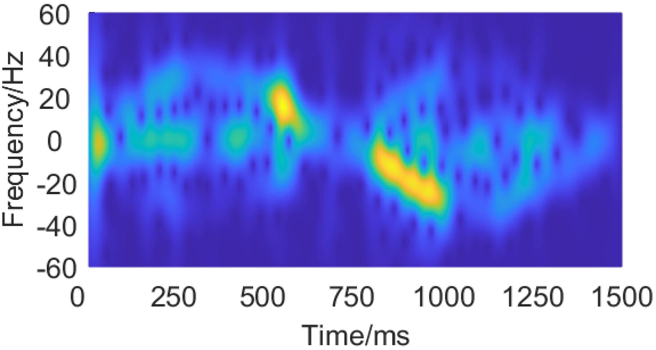 Fig. 18. The measured spectrogram of a pushing and pulling gesture.
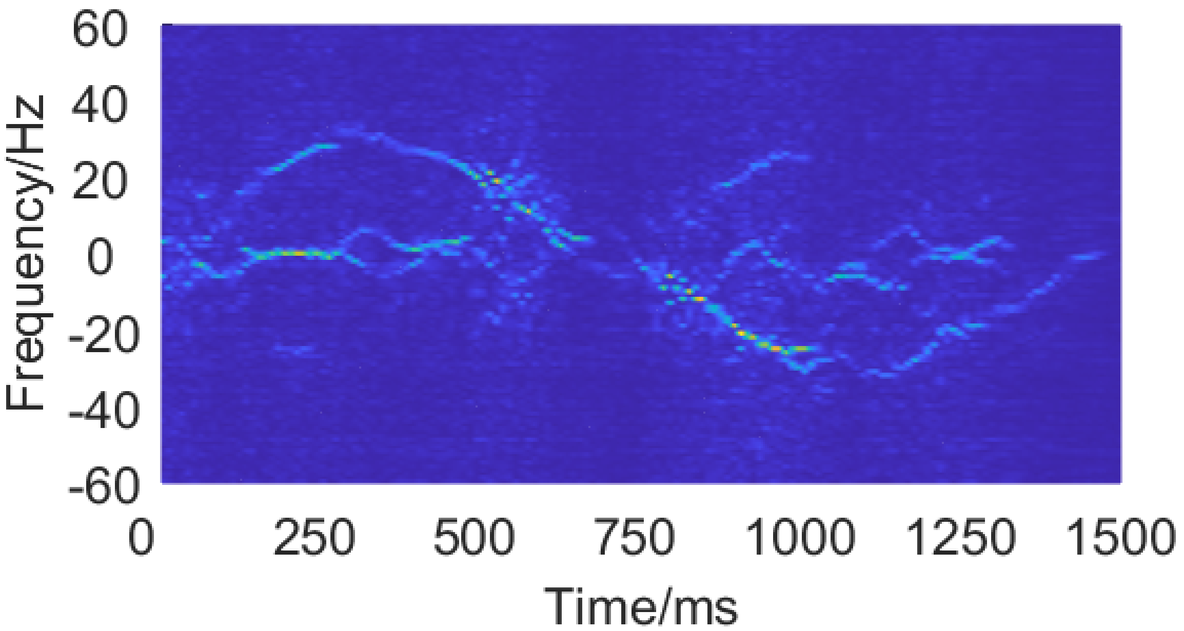 Fig. 19. The enhanced spectrogram from the SEN of a pushing and pulling gesture.
- Wenjun Jiang, Hongfei Xue, Chenglin Miao, Shiyang Wang, Sen Lin, Chong Tian, Srinivasan Murali, Haochen Hu, Zhi Sun, and Lu Su. 2020. Towards 3D Human Pose Construction Using Wifi. In Proceedings of the ACM MobiCom.↩
- Mingmin Zhao, Yonglong Tian, Hang Zhao, Mohammad Abu Alsheikh, Tianhong Li, Rumen Hristov, Zachary Kabelac, Dina Katabi, and Antonio Torralba. 2018. RF-Based 3D Skeletons. In Proceedings of the ACM SIGCOMM.↩
- Yue Zheng, Yi Zhang, Kun Qian, Guidong Zhang, Yunhao Liu, Chenshu Wu, and Zheng Yang. 2019. Zero-Effort Cross-Domain Gesture Recognition with Wi-Fi. In Proceedings of the ACM MobiSys.↩
- Zheng Yang, Yi Zhang, Guidong Zhang, and Yue Zheng. 2020. Widar 3.0: WiFi-based Activity Recognition Dataset. https://doi.org/10.21227/7znf-qp86↩
- François Chollet et al. 2015. Keras. https://github.com/fchollet/keras.↩
- Wenjun Jiang, Chenglin Miao, Fenglong Ma, Shuochao Yao, Yaqing Wang, Ye Yuan, Hongfei Xue, Chen Song, Xin Ma, Dimitrios Koutsonikolas, Wenyao Xu, and Lu Su. 2018. Towards Environment Independent Device Free Human Activity Recognition. In Proceedings of ACM MobiCom.↩