CSI Feature Extraction

tip

All the code and data in this tutorial are available. Click here to download it!

The CSI features lay the fundation of wireless sensing. In particular, for different sensing tasks, choosing the most appropriate features can effectively improve the system performance. In addition, the quality of the extracted features determines the effectiveness of the sensing system.

For ease of illustration, code implementation used for feature extraction is provided below, which is a main function to call different function in the following subsections.

%{
  CSI Feature Extraction for Wi-Fi sensing.  
  - Input: csi data used for calibration, and csi data that need to be sanitized.
  - Output: sanitized csi data.

  To use this script, you need to:
  1. Make sure the csi data have been saved as .mat files.
  2. Check the .mat file to make sure they are in the correct form. 
  3. Set the parameters.
  
  Note that in this algorithm, the csi data should be a 4-D tensor with the size of [T S A L]:
  - T indicates the number of csi packets;
  - S indicates the number of subcarriers;
  - A indicates the number of antennas (i.e., the STS number in a MIMO system);
  - L indicates the number of HT-LTFs in a single PPDU;
  Say if we collect a 10 seconds csi data steam at 1 kHz sample rate (T = 10 * 1000), from a 3-antenna AP (A = 3),  with 802.11n standard (S = 57 subcarrier), without any extra spatial sounding (L = 1), the data size should be [10000 57 3 1].
%}

clear all;
addpath(genpath(pwd));

%% 0. Set parameters.
% Path of the raw CSI data.
src_file_name = './data/csi_src_test.mat';

% Speed of light.
global c;
c = physconst('LightSpeed');
% Bandwidth.
global bw;
bw = 20e6;
% Subcarrier frequency.
global subcarrier_freq;
subcarrier_freq = linspace(5.8153e9, 5.8347e9, 57);
% Subcarrier wavelength.
global subcarrier_lambda;
subcarrier_lambda = c ./ subcarrier_freq;

% Antenna arrangement.
antenna_loc = [0, 0, 0; 0.0514665, 0, 0; 0, 0.0514665, 0]';
% Set the linear range of the CSI phase, which varies with NIC types.
linear_interval = (20:38)';

%% 1. Read the csi data for calibration and sanitization.
% Load the raw CSI data.
csi_src = load(src_file_name).csi;      % Raw CSI.

%% 2. Perform various wireless sensing tasks.
% Test example 1: angle/direction estimation with imperfect CSI.
[packet_num, subcarrier_num, antenna_num, ~] = size(csi_src);
aoa_mat = naive_aoa(csi_src, antenna_loc, zeros(3, 1));
aoa_gt = [0; 0; 1];
error = mean(acos(aoa_gt' * aoa_mat));
disp("Angle estimation error: " + num2str(error));

% Test example 2: distance estimation with CSI.
tof_mat = naive_tof(csi_src);
est_dist = mean(tof_mat * c, 'all');
disp("The ground truth distance is: 10 m");
disp("The estimated distance is: " + num2str(est_dist) + " m");

Time of Flight

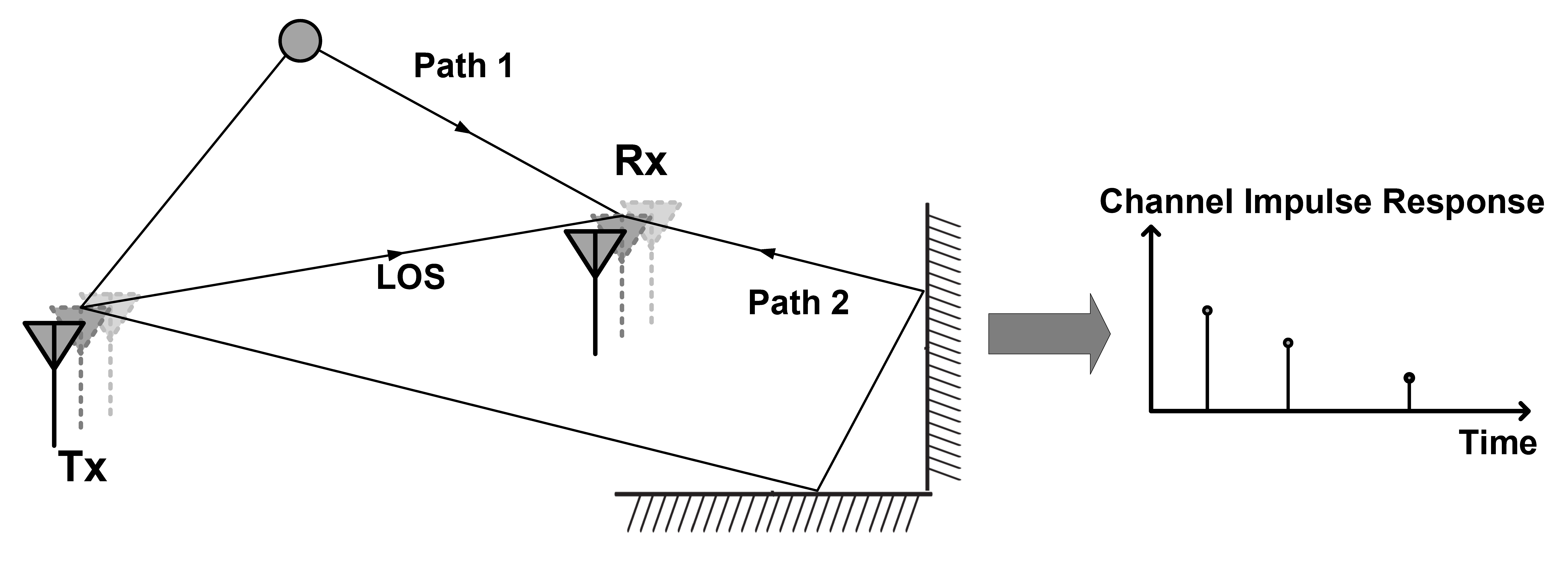
Fig. 5. The relationship between ToF and CIR.

ToF is the time duration the signal propagates from the transmitter to the receiver along a specific path. Given the frequency $f$, the phase shift introduced by the ToF $\tau$ is:

$$\phi_{\mathrm{ToF}} = -2\pi f\tau. \tag{13}$$

As the superimposition of multipath signals, CSI can be represented based on the ray-tracing model:

$$H(f)=\sum_{n=1}^{N}\alpha_{n}e^{-j2\pi f\tau_n} \tag{14}$$

where $N$ is the total number of multipath, and $\alpha_n$ and $\tau_n$ are the complex attenuation factor and time of flight (ToF) for the $n^{th}$ path, respectively. Theoretically, the ToF of all paths can be identified in CIR, which can be calculated by applying the inverse Fourier transform to CSI samples of all subcarriers. However, since the transmitter and the receiver lack synchronization, non-zero temporal shifts exist in CIR, and the absolute ToF is typically not accurate enough. The limited bandwidth also constrains the time resolution, causing meter-level ToF ambiguity The relationship between signal propagation path, ToF, and CIR is shown in Figure. 5.

The following function naive_tof intends to extract the ToF of the strongest path (typically the shortest path) based on inverse Fourier transform.

function [tof_mat] = naive_tof(csi_data)
    % naive_tof
    % Input:
    %   - csi_data is the CSI used for ranging; [T S A E]
    %   - ifft_point and bw are the IFFT and bandwidth parameters;
    % Output:
    %   - tof_mat is the rough time-of-flight estimation result; [T A]

    global c, bw;
    [pakcet_num, subcarrier_num, antenna_num, extra_num] = size(csi_data);
    ifft_point = power(2, ceil(log2(subcarrier_num)));
    % Get CIR from each packet and each antenna by ifft(CFR);
    cir_sequence = zeros(packet_num, antenna_num, extra_num, ifft_point);

    for p = 1:packet_num
        for a = 1:antenna_num
            for e = 1:extra_num
                cir_sequence(p, a, e, :) = ifft(csi_data(p, :, a, e), ifft_point);
            end
        end
    end
    cir_sequence = squeeze(mean(cir_sequence, 4)); % [T ifft_point A]
    half_point = ifft_point / 2;
    half_sequence = cir_sequence(:, 1:half_point, :); % [T half_point A]
    peak_indices = zeros(packet_num, antenna_num); % [T A]
    for p = 1:pakcet_num
        for a = 1:antenna_num
            [~, peak_indices(p, a)] = max(half_sequence, [], 2);
        end
    end
    % Calculate ToF;
    tof_mat = peak_indices .* subcarrier_num ./ (ifft_point .* bw); % [T A]
end

Angle of Arrival and Angle of Departure

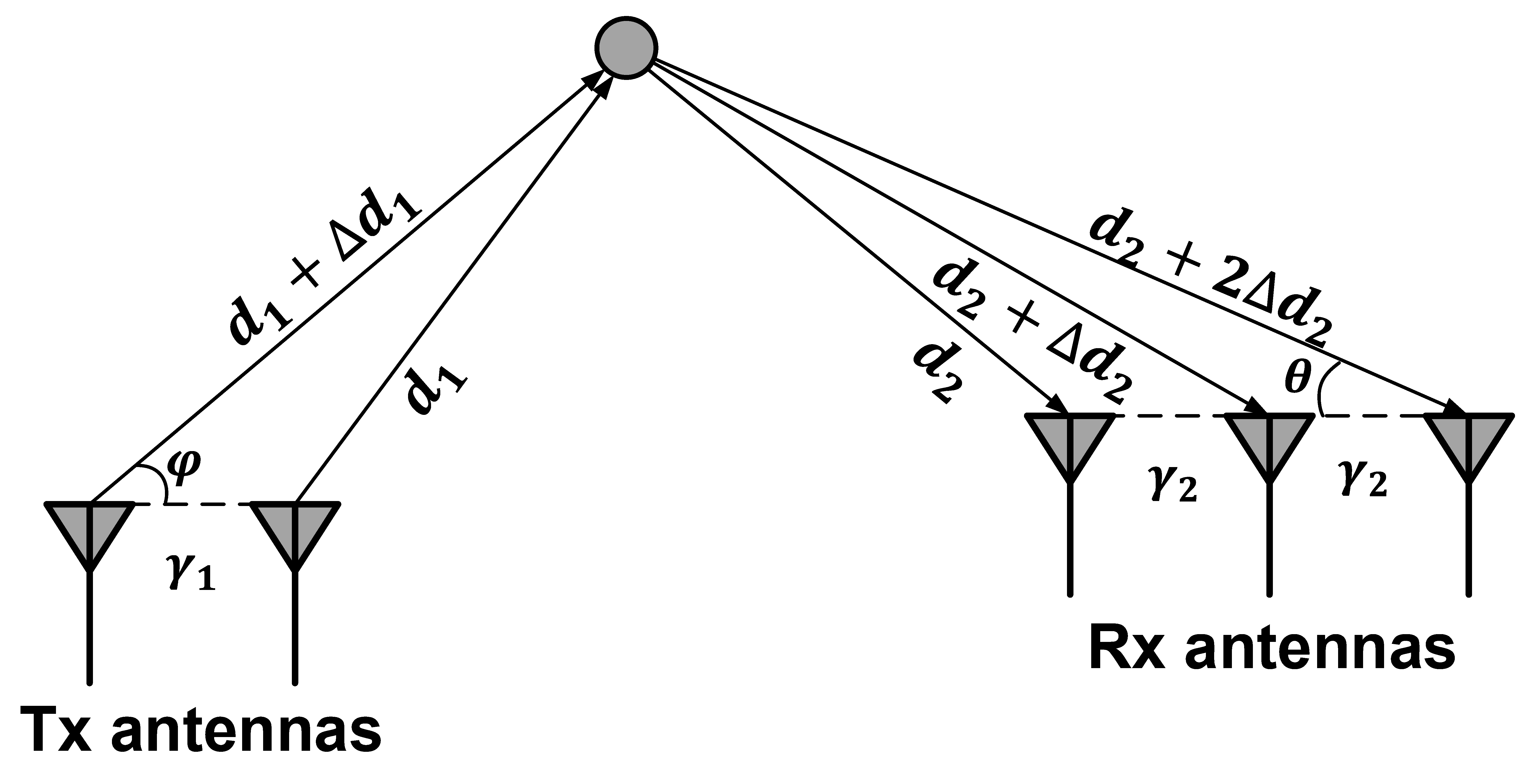
Fig. 6. Angle of Arrival and Angle of Departure.

When a NIC equipes with multiple antennas, a local coordinate at the device can be created. As shown in Figure. 6, for a transmitter, the angle of departure (AoD) $\varphi$ represents the direction in the local coordinate along which the transmitted signal is emitted. For a receiver, the angle of arrival (AoA) $\theta$ represents the direction in the local coordinate along which the received signal is captured. Since the antennas are spatially separated, non-zero phase shifts between antennas are introduced. The phase shifts depend on the AoA/AoD. Specifically, suppose the relative location between two antennas is $\bm{\Delta{l}}=(\Delta_x, \Delta_y)$ and the unit direciton vector of AoA is $\bm{e}=(\cos\theta, \sin\theta)$, the phase shift between the two antennas is:

$$\tag{15} \phi_{\mathrm{AoA}} = \frac{2\pi}{\lambda}\bm{\Delta{l}}\cdot\bm{e}$$

Then CSI can be modeled as:

$$\tag{16} H(k)=\sum_{n=1}^{N}\alpha_{n}e^{-j\frac{2\pi}{\lambda}\bm{\Delta{l}}\cdot\bm{e}}$$

where $k$ represents the $k^{th}$ antenna at the receiver. The same model applies to the AoD at the trasmitter side and the 3D space with azimuth and elevation angles.

In practice, algorithms such as Capon ¹ and MUSIC ² can be used to estimate the AoA/AoD of multiple paths from the CSI of the antenna array.

MUSIC analyses the incident signals on multiple antennas to find out the AoA of each signal.

Specifically, suppose $D$ signals $F_{1},\cdots,F_{D}$ arrive from directions $\theta_{1},\cdots,\theta_{D}$ at $M > D$ antennas.

The received signal at the $k^{th}$ antenna element, denoted as $X_{k}$, is a linear combination of the $D$ incident wavefronts and noise $W_{k}$:

$$\tag{17} \left[\begin{array}{c} X_{1} \\ X_{2} \\ \vdots \\ X_{M} \end{array}\right]=\left[\begin{array}{llll} a\left(\theta_{1}\right) & a\left(\theta_{2}\right) & \ldots & a\left(\theta_{D}\right) \end{array}\right]\left[\begin{array}{c} F_{1} \\ F_{2} \\ \vdots \\ F_{D} \end{array}\right]+\left[\begin{array}{c} W_{1} \\ W_{2} \\ \vdots \\ W_{M} \end{array}\right],$$

or

$$\tag{18} X=A F+W,$$

where $\bm{a}(\theta_{k})$ is the array steering vector that characterizes added phase (relative to the first antenna) of each receiving component at the $k^{th}$ antenna, and $\bm{A}$ is the matrix of steer vectors.

As shown in Figure. 6, for a linear antenna array with elements well synchronized,

$$\tag{19} \bm{a}(\theta)=\left[ \begin{array}{c} 1\\ e^{-j\frac{2\pi}{\lambda}\bm{\Delta{l(1)}}\cdot\bm{e}}\\ e^{-j\frac{2\pi}{\lambda}\bm{\Delta{l(2)}}\cdot\bm{e}}\\ \vdots\\ e^{-j\frac{2\pi}{\lambda}\bm{\Delta{l(M-1)}}\cdot\bm{e}} \end{array} \right].$$

Suppose $W_{k}\sim N(0, \sigma^{2})$, and $F_k$ is a wide-sense stationary process with zero mean value, the $M\times M$ covariance matrix of the received signal vector $\bm{X}$ is:

$$\tag{20} \begin{aligned} S &=\overline{X X^{\mathrm{H}}} \\ &=A \overline{F F^{\mathrm{H}}} A^{\mathrm{H}}+\overline{W W^{\mathrm{H}}} \\ &=A P A^{\mathrm{H}}+\sigma^{2} I, \end{aligned}$$

where $\bm{P}$ is the covariance matrix of transmission vector $\bm{F}$. The notation $(\cdot)^{\mathrm{H}}$ represents conjugate transpose and $\overline{(\cdot)}$ represents expectation.

The covariance matrix $\bm{S}$ has $M$ eigenvalues $\lambda_{1},\cdots,\lambda_{M}$ associated with $M$ eigenvectors $\bm{e}_{1},\bm{e}_{1},\cdots,\bm{e}_{M}$. Sorted in a non-descending order, the smallest $M-D$ eigenvalues correspond to the noise while the rest $D$ correspond to the $D$ incident signals.

In other word, the $M$-dimension space can be divided into two orthogonal subspace, the noise subspace $\bm{E}_{N}$ expanded by eigenvectors $\bm{e}_{1},\cdots,\bm{e}_{M-D}$, and the signal subspace $\bm{E}_{S}$ expanded by eigenvectors $\bm{e}_{M-D+1},\cdots,\bm{e}_{M}$ (or equivalently $D$ array steering vector $\bm{a}(\theta_{1}),\cdots,\bm{a}(\theta_{D})$).

To solve for the array steering vectors (thus AoA), MUSIC plots the reciprocal of squared distance $Q(\theta)$ for points along the $\theta$ continue to the noise subspace as a function of $\theta$:

$$\tag{21} Q(\theta)=\frac{1}{\bm{a}^{\mathrm{H}}(\theta)\bm{E}_{N}\bm{E}_{N}^{\mathrm{H}}\bm{a}(\theta)}$$

This yields peaks in $Q(\theta)$ at the bearing of incident signals. It is similar to apply MUSIC algorithm for AoD spectrum estimation.

The following function naive_aoa intends to estimate the 3D AoA based on the phase difference, which is similar to Eqn. 15. Note that the following algorithm only considers one path, and thus cannot be applied to mutlipath signals.

function [aoa_mat] = naive_aoa(csi_data, antenna_loc, est_rco)
    % naive_aoa
    % Input:
    %   - csi_data is the CSI used for angle estimation; [T S A E]
    %   - antenna_loc is the antenna location arrangement with the first antenna as a reference; [3 A]
    %   - est_rco is the estimated radio chain offset; [A 1]
    % Output:
    %   - aoa_mat is the angle estimation result; [3 T]

    global subcarrier_lambda;
    [packet_num, subcarrier_num, antenna_num, extra_num] = size(csi_data);
    csi_phase = unwrap(angle(csi_data), [], 2);    % [T S A E]
    % Get the antenna vector and its length.
    ant_diff = antenna_loc(:, 2:end) - antenna_loc(:, 1); % [3 A-1]
    ant_diff_length = vecnorm(ant_diff); % [1 A-1]
    ant_diff_normalize = ant_diff ./ ant_diff_length; % [3 A-1]
    % Calculate the phase difference.
    phase_diff = csi_phase(:, :, 2:end, :) - csi_phase(:, :, 1, :) - permute(est_rco(2:end, :), [4 3 1 2]); % [T S A-1 E]
    phase_diff = unwrap(phase_diff, [], 2);
    phase_diff = mod(phase_diff + pi, 2 * pi) - pi;
    % Broadcasting is performed, get the value of cos(theta) for each packet and each antenna pair.
    cos_mat = subcarrier_lambda .* phase_diff ./ (2 .* pi .* permute(ant_diff_length, [3 1 2])); % [T S A-1 E]
    cos_mat_mean = squeeze(mean(cos_mat, [2 4])); % [T A-1]
    % Symbolic nonlinear optimization are performed.
    syms x y
    % aoa_sol = [x;y;(1-sqrt(x^2 + y^2))];
    aoa_init = [sqrt(1/3);sqrt(1/3);sqrt(1/3)];
    aoa_mat_sol = zeros(3, packet_num);
    options = optimoptions('lsqnonlin', 'Algorithm', 'levenberg-marquardt', 'Display', 'none');
    parfor p = 1:packet_num
       cur_nonlinear_func = @(aoa_sol)ant_diff_normalize' * aoa_sol - cos_mat_mean(p, :)';
       cur_aoa_sol = lsqnonlin(cur_nonlinear_func, aoa_init, [], [], options);
       aoa_mat_sol(:, p) = cur_aoa_sol;
    end
    aoa_mat = aoa_mat_sol ./ vecnorm(aoa_mat_sol); % [3 T]
end

Phase Shift

Fig. 7. Phase shift spectrum (a.k.a Doppler spectrum) of three different moving path.

Non-zero phase shift $\Delta \phi$ across different packets is caused by the relative movement of the transmitter, receiver, or objects in the propagation path of the signal. It equals the changing rate of the path length of the signal.
When multiple packets are received in sequence, the CSI corresponding to the $i^{th}$ received packet is:

$$H(i) = \sum_{n=1}^{N}\alpha_{n}(i)e^{j\phi_{n}(i)}, \tag{22}$$

where $\phi_{n}$ is the phase of the $n^{th}$ path ³. Extract the phase of the the $n^{th}$ path in packet $i$ and $i+1$ respectively, and calculate the phase shift as:

$$\Delta \phi_{n}(i) = \phi_{n}(i+1) - \phi_{n}(i). \tag{23}$$

Intuitively, the phase difference indicates the distance change of the $n^{th}$ path between two consecutive packets: $\Delta d_{n}(i) = \frac{\Delta \phi_{n}(i)}{2 \pi} \lambda$.

Take a step further, and apply the short-time Fourier transform (STFT) within a sliding window, we can get the spectrum as shown in Figure. 7. The frequency axis reveals the change rate of consecutive CSI data, and implicitly contains the path length change rate. Figure. 7 demonstrates the phase shift spectrum (or the Doppler Spectrum) for three different moving paths.

The following function naive_stft calculates the short-time Fourier transform of a series of CSI data. The generated spectrum can be used effectively for many wireless sensing tasks, like gesture recognition and fall detection.

function stft_mat = naive_spectrum(csi_data, sample_rate, visable)
    % naive_spectrum
    % Input:
    %   - csi_data is the CSI used for STFT spectrum generation; [T S A L]
    %   - sample_rate determines the resolution of the time-domain and
    %   frequency-domain;
    % Output:
    %   - stft_mat is the generated STFT spectrum; [sample_rate/2 T]

    % Conjugate multiplication.
    csi_data = mean(csi_data .* conj(csi_data), [2 3 4]);
    % Calculate the STFT and visualization.
    stft_mat = stft(csi_data, sample_rate);
    % Visualization (optional).
    if visable
        stft(csi_data, sample_rate);
    end
end

Body-coordinate Velocity Profile

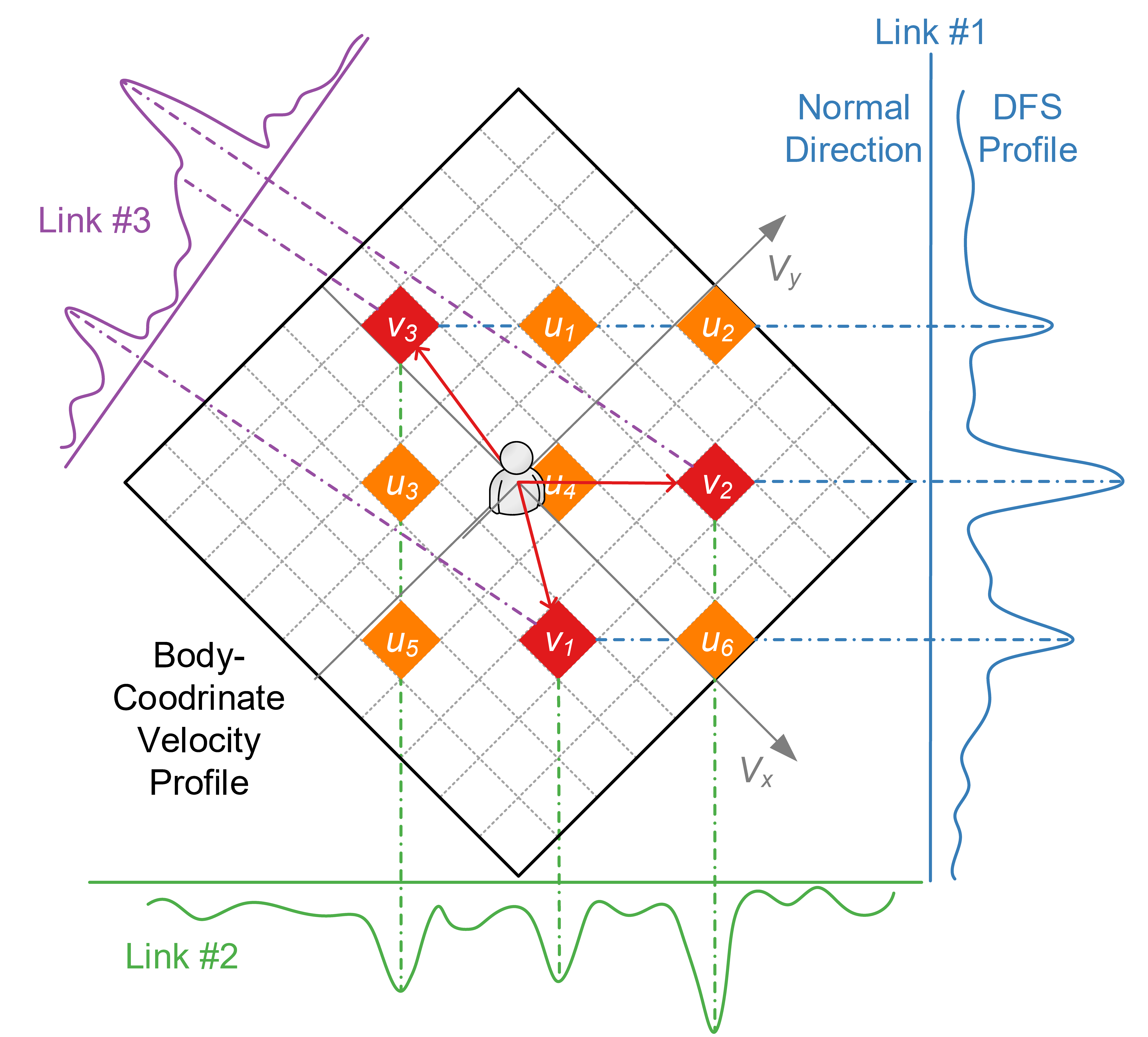
Fig. 8. Relationship between the BVP and Doppler spectrum. Each velocity component in BVP is projected onto the normal direction of a link, and contributes to the power of the corresponding radial velocity component in the Doppler spectrum.

The limitation of the aforementioned spectrum is that, even the spectrum corresponding to the same activity will be different when the user moves at different locations or orientations relative to the Wi-Fi links. To resolve this problem, Widar3.0 ⁴ proposes a domain-independent signal feature BVP (body-coordinate velocity profile) to characterize human activities.

The basic idea of BVP is shown in Figure. 8. A BVP $\bm{V}$ is quantized as a discrete matrix with dimension as velocity components decomposed along each axis of the body coordinates. For convenience, we establish the local body coordinates whose origin is the location of the person and positive x-axis aligns with the orientation of the person. The person's location and orientation should be provided manually. Currently, it is assumed that the global location and orientation of the person are available. Then the known global locations of wireless transceivers can be transformed into the local body coordinates. Thus, for better clarity, all locations and orientations used in the following derivation are in the local body coordinates. Suppose the locations of the transmitter and the receiver of the $i^{th}$ link are $\vec{l}_{t}^{(i)}=(x_{t}^{(i)},y_{t}^{(i)})$, $\vec{l}_{r}^{(i)}=(x_{r}^{(i)},y_{r}^{(i)})$, respectively, then any velocity components $\vec{v}=(v_x, v_y)$ around the human body (\ie, the origin) will contribute its signal power to some frequency component, denoted as $f^{(i)}(\vec{v})$, in the Doppler spectrum of the $i^{th}$ link ⁵:

$$\tag{24} f^{(i)}(\vec{v})=a_{x}^{(i)}v_x+a_{y}^{(i)}v_y,$$

where $a_{x}^{(i)}$ and $a_{y}^{(i)}$ are coefficients determined by locations of the transmitter and the receiver:

$$\begin{aligned} \tag{25} a_{x}^{(i)} &=\frac{1}{\lambda}\left(\frac{x_{t}^{(i)}}{\left\|\vec{l}_{t}^{(i)}\right\|_{2}}+\frac{x_{r}^{(i)}}{\left\|\vec{l}_{r}^{(i)}\right\|_{2}}\right), \\ a_{y}^{(i)} &=\frac{1}{\lambda}\left(\frac{y_{t}^{(i)}}{\left\|\vec{l}_{t}^{(i)}\right\|_{2}}+\frac{y_{r}^{(i)}}{\left\|\vec{l}_{r}^{(i)}\right\|_{2}}\right), \end{aligned}$$

where $\lambda$ is the wavelength of Wi-Fi signal.

As static components with zero Doppler spectrum (\eg, the line of sight signals and dominant reflections from static objects) are filtered out before the Doppler spectrum are calculated, only signals reflected by the person are retained. Besides, when the person is close to the Wi-Fi link, only signals with one-time reflection have prominent magnitudes ⁶. Thus, Eqn.24 holds valid for the gesture recognition scenario. From the geometric view, Eqn.24 means that the 2-D velocity vector $\vec{v}$ is projected on a line whose direction vector is $\bm{d}^{(i)}=(-a_{y}^{(i)}, a_{x}^{(i)})$. Suppose the person is on an ellipse curve whose foci are the transmitter and the receiver of the $i^{th}$ link, then $d^{(i)}$ is indeed the average direction of the ellipse at the person's location. Figure. 8 shows an example where the person generates three velocity components $\vec{v}_j, j=1,2,3$, and projection of the velocity components on the Doppler spectrum of three links.

Since coefficients $a_{x}^{(i)}$ and $a_{y}^{(i)}$ only depend on the location of the $i^{th}$ link, the relation of projection of the BVP on the $i^{th}$ link is fixed. Specifically, an assignment matrix $\bm{A}^{(i)}_{F\times N^2}$ can be defined:

$$\tag{26} A_{j, k}^{(i)}= \begin{cases}1 & f_{j}=f^{(i)}\left(\vec{v}_{k}\right) \\ 0 & \text { else }\end{cases},$$

where $f_j$ is the $j^{th}$ frequency sampling point in the Doppler spectrum, and $\vec{v}_k$ is velocity component corresponding to the $k^{th}$ element of the vectorized BVP $\bm{V}$. Thus, the relation between Doppler spectrum profile of the $i^{th}$ link and the BVP can be modeled as:

$$\tag{27} \bm{D}^{(i)}=c^{(i)}\bm{A}^{(i)}\bm{V},$$

where $c^{(i)}$ is the scaling factor due to propagation loss of the reflected signal.

Due to the sparsity of BVP, compressed sensing ⁷ technique can be adopted to formulate the estimation of BVP as an $l_0$ optimization problem:

$$\tag{28} {\rm min}_{V}\sum_{i=1}^{M}|{\rm EMD}(\bm{A}^{(i)}\bm{V}, \bm{D}^{i})|+\eta\|V\|_0,$$

where $M$ is the number of Wi-Fi links.

The sparsity of the number of the velocity components is coerced by the term $\eta\|V\|_0$, where $\eta$ represents the sparsity coefficients and $\|\cdot\|_0$ is the number of non-zero velocity components.

${\rm EMD}(\cdot,\cdot)$ is the Earth Mover's Distance ⁸ between two distributions. The selection of EMD rather than Euclidean distance is mainly due to two reasons. First, the quantization of BVP introduces approximation error, \ie, projection of velocity components to the Doppler spectrum bin might be adjacent to the true one. Such quantization error can be relieved by EMD, which takes the distance between bins into consideration. Second, there are unknown scaling factors between the BVP and Doppler spectrum, making the Euclidean distance inapplicable.

---

1. J. Capon. 1969. High-resolution frequency-wavenumber spectrum analysis. Proc. IEEE (1969).↩
2. R. Schmidt. 1986. Multiple emitter location and signal parameter estimation. IEEE Transactions on Antennas and Propagation (1986).↩
3. Guoxuan Chi, Zheng Yang, Jingao Xu, Chenshu Wu, Jialin Zhang, Jianzhe Liang, and Yunhao Liu. 2022. Wi-drone: Wi-Fi-based 6-DoF Tracking for Indoor Drone Flight Control. In Proceedings of the ACM MobiSys.↩
4. Yue Zheng, Yi Zhang, Kun Qian, Guidong Zhang, Yunhao Liu, Chenshu Wu, and Zheng Yang. 2019. Zero-Effort Cross-Domain Gesture Recognition with Wi-Fi. In Proceedings of the ACM MobiSys.↩
5. Kun Qian, Chenshu Wu, Zheng Yang, Yunhao Liu, and Kyle Jamieson. 2017. Widar: Decimeter-Level Passive Tracking via Velocity Monitoring with Commodity Wi-Fi. In Proceedings of the ACM MobiHoc.↩
6. Kun Qian, Chenshu Wu, Yi Zhang, Guidong Zhang, Zheng Yang, and Yunhao Liu. 2018. Widar2.0: Passive human tracking with a single wi-fi link. Proceedings of the ACM MobiSys (2018).↩
7. David L Donoho. 2006. Compressed sensing. IEEE Transactions on information theory (2006).↩
8. Yossi Rubner and Carlo Tomasi. 2001. The earth mover’s distance. In Perceptual Metrics for Image Database Navigation. Springer.↩